The skin is an electrical organ, and it produces slow drifts in voltage that are picked up by our EEG electrodes. These skin potentials can cause the voltage to gradually change by hundreds of microvolts over a period of a few minutes. To get a better look at the skin potentials, go to the EEG plotting window that you opened in the previous exercise (or open the window again), and change the settings as follows:
Go to time zero by putting a zero in the text box between the < and > buttons in the plot window.
Set the vertical gain to 100 (using the little text box near the bottom of the plot window).
Set the time range to 400 seconds using Settings > Time range to display in the plot window.
Stretch the window as wide as you can so that it looks something like the top window in Screenshot 2.4.
Screenshot 2.4
Looks pretty weird, doesn’t it? The first thing you should look at is the event codes (the vertical lines). The N400 experiment lasted about 6 minutes, and you’re looking at the entire recording, so there are lots of event codes. Notice that there are 6 clusters of event codes, separated by gaps of approximately 7 seconds. The 120 trials in this experiment were divided into 6 blocks of 20 trials each, with a short rest break after each block. I find that participants can maintain their attention better if we use a large number of short blocks, each followed by a brief break, so this experiment was broken up into short blocks that lasted only about a minute each.
Now take a look at the EEG waveforms. You can now see that the voltage is gradually drifting over time. It drifts upward in some channels and downward in others. Most of the channels change by well over 100 µV over the course of this 400-second period. These drifts are mainly caused by electrical potentials in the skin that are picked up by the EEG electrodes (see Chapter 5 in Luck, 2014 for more details).
These drifts can make it difficult to obtain reliable ERP differences across conditions, and it’s usually a good idea to filter them out. To accomplish this, we apply a high-pass filter, which filters out low frequencies and passes high frequencies. Here, we’ll use the filter settings that I recommend for most studies of cognitive and affective processes, which has a half-amplitude cutoff at 0.1 Hz and a slope of 12 dB/octave. If you don’t know what these parameters mean, don’t worry – we’ll cover them in Chapter 4. You can also find a broad conceptual overview of filters in Chapter 7 of Luck (2014) and a more detailed mathematical treatment in Chapter 12 of Luck (2014).
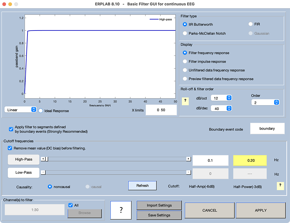
Now let’s get rid of these drifts with a high-pass filter. Leave the current plotting window open, and go to EEGLAB > ERPLAB > Filter & Frequency Tools > Filters for EEG data. You’ll see ERPLAB’s filtering GUI, which is big and complicated (because filters have a lot of different options). We’ll explain these options in a later chapter, but for this exercise you should just make sure that everything is set to match Screenshot 2.5. Most importantly, make sure the High-Pass button is selected with a half-amplitude cutoff of 0.1 Hz, and the Low-Pass button is not selected (these button are a slightly darker gray when selected).
Getting an Error Message?
Did you get an error message when you launched the filtering tool? If so, the message probably said that you're missing the Signal Processing Toolbox. This toolbox comes from the makers of Matlab and is required for certain ERPLAB processes, such as filtering. Depending on your institution's Matlab license, it may be free or it may require an extra fee.
You can see what toolboxes are installed by typing ver on the Matlab command line. If you don't have the Signal Processing Toolbox and you don't know how to get it and/or install it, contact your institution's IT support department for assistance.
Screenshot 2.5
Saving the New Dataset
Once all the parameters are set, click the APPLY button. You’ll then see the window shown in Screenshot 2.6, which asks What do you want to do with the new dataset? In EEGLAB and ERPLAB, most operations that modify a dataset will actually create a new dataset. That way, if you make a mistake or change your mind, you can easily go back to the previous dataset. These datasets are stored in memory, where they’re listed in the Datasets menu, and you can also save them to your hard drive if you want. The top text box in Screenshot 2.6 allows you to specify the name of the dataset (which will be the name shown in the Datasets menu). You can use any name you like, but ERPLAB will give you a suggestion (which is the name of the original dataset with a suffix that indicates the nature of the processing step, such as _filt for filtering).
If you want to save the dataset as a file on your hard drive, check the box next to Save it as a file and type in the name that will be used for this file. The name of the dataset in memory doesn’t have to be the same as the filename, but it can be confusing if the name in memory is different from the filename. I usually just select the name of the dataset from the top text box, copy it into the clipboard, and the paste it into the second text box. Note that if you don’t save the dataset as a file now, you can save it later with EEGLAB > File > Save current dataset as. You’ll need the new filtered dataset for the next exercise, so you should save it as a file if you’re not going to do the next exercise right away.
Once you have everything set in this window, click OK. You’ve now created a new dataset with the filtered data. The previous dataset was named 6_N400_preprocessed, and the new one should be named 6_N400_preprocessed_filt. If you look in the Datasets menu in the main EEGLAB GUI, you should see both of these datasets listed, with the new one checked.
Screenshot 2.6
Looking at the Filtered Data
Now that you’ve saved the dataset, plot the filtered data with EEGLAB > Plot > channel data (scroll). Set it up like the plotting window that shows the unfiltered data (remove the DC offset, set the vertical gain to 100, set the time range to 400 second, and stretch the window to the same width). It should look something like the bottom window in Screenshot 2.4. The slow drifts are now gone, and the data look much more orderly. We’ve now gotten rid of a major source of artifactual activity from the EEG, which improve our ability to obtain robust, reliable ERP effects.
Now change the time period to display to be 10 seconds instead of 400 seconds for both the unfiltered and filtered data. Because you’re still removing the DC offset and the drifts are slow, the filtered and unfiltered data don’t look as radically different with this 10-second time scale as they did with the 400-second time scale. But if you look carefully (especially at the PO3 channel), you’ll see that there is some drift in the unfiltered data that is absent in the filtered data. You can also see that all the faster deflections in the data are present in both the filtered and unfiltered waveforms. So, the high-pass filter has largely eliminated the slow drifts but has had minimal effect on the other features of the EEG. We’ll take a closer look at filters in Chapter 4.
You’ll need the filtered dataset for the next exercise. If you’re going to do the next exercise right away, just leave EEGLAB open (but you can close the two plotting windows). If you’re not going to do it right away, you can save the filtered dataset as a file on your hard drive by selecting EEGLAB > File > Save current dataset as.