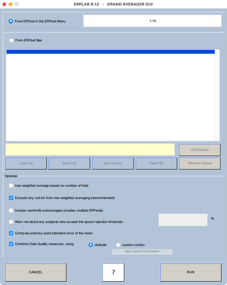
Although it’s important to look at the single-participant ERP waveforms, it will be easier to see subtle effects by averaging the waveforms across participants to create grand average waveforms for each bin. To do this, make sure that the ERPsets from all 10 participants are loaded (which you can verify by looking at the ERPsets menu), and then select EEGLAB > ERPLAB > Average across ERPsets (Grand Average). A new window will open that look something like Screenshot 3.3.
Screenshot 3.3
You need to specify which ERPsets will be averaged together. You can do this either by specifying a set of ERPsets that have already been loaded (using the ERPset numbers in the ERPsets menu) or by specifying the filenames for ERPsets that have been stored in files. In this exercise, we’ll specify the ERPsets that have already been loaded. If you have only the 10 ERPsets from our 10 example participants in your ERPsets menu, you can specify 1:10 (as in Screenshot 3.3). In Matlab, you can indicate a list of consecutive numbers by providing the first and last numbers, separated by a colon. So, 1:10 is equal to 1 2 3 4 5 6 7 8 9 10. If these aren’t the right ERPsets (because you have others also loaded into ERPLAB), just provide a list of the ten numbers for the ERPsets you want to average together.
You can leave the other options set to their default values (making sure that they match Screenshot 3.3). Then click RUN. You’ll then see the usual window for saving the new ERPset that you’ve created. Name it Grand_N400 (and save it as a file so that you have it for the subsequent exercises). You should now see Grand_N400 in the ERPsets menu.
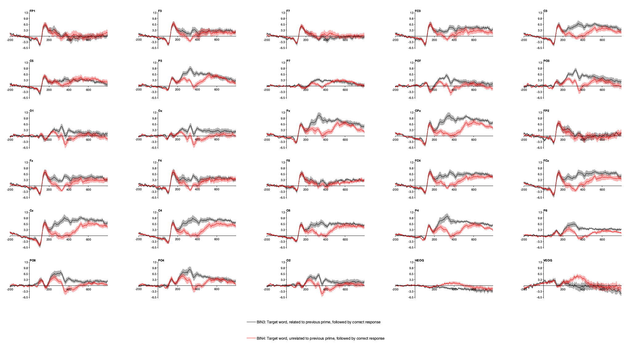
Now, plot the ERPs from Bins 3 and 4 (using EEGLAB > ERPLAB > Plot ERPs > Plot ERP waveforms). But let’s add something new: Tick the box labeled show standard error (and make sure that the transparency level is set to 0.7). You should see something like Screenshot 3.4, with a more negative voltage for the unrelated targets than for the related targets at CPz and surrounding electrode sites. The light shading around the waveforms is the standard error of the mean at each time point (see the box below for more information).
Screenshot 3.4
Now plot Bins 1 and 2. The waveforms for these bins should be lying right on top of each other, with any differences being small relative to the SEM. Remember, these are the bins for primes that are followed by related versus unrelated targets, and unless the participants have ESP, they can’t differ as a function of something that happens later. As a result, any differences between them are simply a result of noise.
Finally, take a look at the aSME data quality values for the grand average (EEGLAB > ERPLAB > Data Quality options > Show Data Quality measures in a table). When you made the grand average, the default settings caused the aSME values from the individual participants to be combined together using something called the root mean square (RMS). This is like taking the average of the single-participant aSME, except that the RMS value is more directly related to the impact of each participant’s data quality to the effect size (see Luck et al., 2021). These aSME values are like a standard error, but they’re the standard error of the mean voltage over a 100-ms time window rather than the SEM at a single time point (see the box below). If you look at the table of aSME values, you’ll see that the values in the N400 time range are around 1.5 µV. That’s reasonably small relative to the large difference in mean voltage between the unrelated and related targets. In other words, the data quality is quite good for our goal of detecting differences between these two types of targets.
Plotting the Standard Error
Plotting the standard error of the mean (SEM) at each time point in an ERP waveform, as in Screenshot 3.4, can be helpful in assessing whether the differences between conditions are reasonably large relative to the variability among participants. These standard error values are just like the error bars that you might see in a bar graph. At each time point, the grand average ERP waveform is simply the mean of the voltage values across participants at that time point. The SEM is just the standard deviation (SD) of the single-participant values divided by the square root of the number of participants (which is exactly how the SEM is usually calculated in other contexts).
You can also see the SEM when you plot a single participant’s averaged ERP waveforms. In this case, the waveform shows the mean across trials rather than the mean across participants, and the SEM reflects the variability across trials rather than the variability across time points.
Although the SEM can be useful, it has some downsides. First, imagine that the voltage at 400 ms is exactly 3µV more negative for unrelated targets than for related targets in every participant (i.e., the experimental effect is extremely consistent across participants). But imagine that the overall voltage at 400 ms is much more positive in some participants than others, leading to quite a bit of variability in the voltage for each condition. Because of this variability, the SEM for each waveform would be quite large at 400 ms. This would make it look like the difference in means between conditions was small relative to the SEM, even though the difference for each participant was extremely consistent. In behavioral research, this problem is addressed by using the within-subjects SEM (Cousineau, 2005; Morey, 2008). ERPLAB doesn’t have this version of the SEM built in, but you can achieve the same result by making a difference wave between the conditions (e.g., unrelated targets minus related targets) and getting the SEM of the difference wave. This is exactly what was done in the grand averages from the full study (see Figure 2.1C in Chapter 2).
Another downside of the SEM is that it can be very large if there is a lot of high-frequency noise in the data, even though this noise has minimal impact when we quantify the N400 as the mean voltage between 300 and 500 ms (as we will do later in this chapter). The aSME value provided in our Data Quality measures does not have this downside, because it provides the standard error of the mean voltage over a time period rather than the standard error of the values at individual time points. See Luck et al. (2021) for a more detailed discussion.