In this exercise, we’re going to repeat the N400 analysis from the previous exercises, but we’re going to make it more complex by measuring and analyzing the N400 at multiple electrode sites. We’ll set this up with two electrode factors: laterality (left hemisphere, midline, and right hemisphere) and anterior-posterior (frontal, central, and parietal). That is, we’ll obtain scores from F3, Fz, F4, C3, Cz, C4, P3, Pz, and P4. When we combine this with the relatedness factor, this will give us a factorial design with three total factors. We won’t include CPz in these analyses because we don’t have electrodes at CP3 and CP4 and we don’t want an unbalanced design.
Launch the Measurement Tool again and set it up exactly as before (Screenshot 3.7) except for the list of channels. If you click the Browse button next to the text box for the channels, you’ll be able to select the nine electrode sites that we want. After you’ve selected them, click OK to go back to the Measurement Tool. You should now see 2 5 7 13 16 17 21 22 24 in the text box. These are the channels we want. You should also change the name of the output file to be mean_amplitude_multiple_channels.txt. Use the Viewer to make sure that everything looks OK, and then click RUN in the Measurement Tool.
Now open the mean_amplitude_multiple_channels.txt file in the Matlab text editor. The text editor doesn’t deal with the tabs very well, so you might want to import the file into Excel instead. Now we have 19 columns: 9 channels x 2 bins plus the ERPset column. Unfortunately, the channels are in the order that they appear in the ERPsets, which is not very convenient. If you’re not sure whether the amplitude scores are correct, you can launch the Measurement Tool again and use the Viewer to see the single-subject scores.
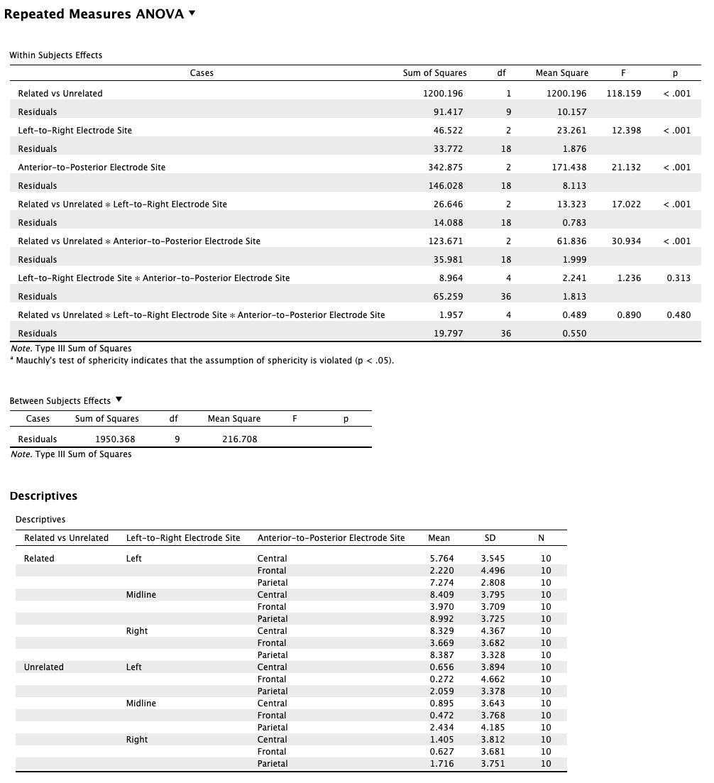
Once you’ve verified that the scores are correct, you can enter the data into a statistical analysis. You should use a 3-way repeated-measures ANOVA with factors of relatedness, laterality, and anterior-posterior. I ran this ANOVA in JASP, and the results are shown in Screenshot 3.9.
Screenshot 3.9
Again, start by looking at the descriptive statistic and make sure they match the grand average waveforms in Screenshot 3.4. For example, in both cases the amplitude for the related trials increases from the frontal to the central and parietal channels, and it tends to be larger for the midline and right-hemisphere channels than for the left-hemisphere channels. You can also see the basic N400 effect in both the grand average waveforms and the group means: the voltage is more negative (less positive) for the unrelated targets than for the related targets.
If you look at the F and p values, you’ll see that the main effect of relatedness (related vs. unrelated) was significant at the p < .001 level. The laterality and anterior-posterior main effects were also significant, and these factors both interacted significantly with relatedness. That is, the difference between related and unrelated words was largest at the sites where the voltage was largest. This pattern of interactions is exactly what would be expected given the multiplicative relationship between the magnitude of an internal ERP generator and the observed scalp distribution (see Chapter 10 in Luck, 2014).
You’ve now completed a fairly sophisticated analysis of the N400 experiment. Congratulations! That was a lot of steps, and it took us two chapters to get to this point.
However, I should note that I don’t generally recommend scoring a component from multiple sites and including electrode site factors in the statistical analysis. The reasoning is described in the text box below. Sometimes it is justifiable, such as when your scientific hypothesis leads to a prediction of different effects over the left and right hemispheres. But unless you have a real reason to compare the effects across electrode sites, it’s usually better to limit your analysis to a single site or create a waveform that averages across multiple sites. We’ll explore the latter option in the next exercise.
Minimizing the Number of Factors in an Analysis
The problem with including one or more electrode site factors is that it leads to a large number of statistical tests, increasing the likelihood that you’ll get one or more significant effects that are a result of random noise in the data. Look at the table of statistics at the top of Screenshot 3.9—how many p values do you see? Seven!
Ordinarily, you would expect a 5% probability that an effect will be significant (p < .05) when the null hypothesis is true. However, if the null hypothesis were true for all seven of these tests, the chance that one or more would be significant (p < .05) would be greater than 30%!
As we increase the number of factors in an ANOVA, the number of main effects and interactions skyrockets, and the odds that one or more will be significant by chance becomes extremely high (Cramer et al., 2015; Frane, 2021). For example, in a 5-way ANOVA, you are more likely than not to obtain a significant-but-bogus-effect. As a result, it is difficult to trust the results of such analyses. My general advice is therefore to minimize the number of factors (see Luck & Gaspelin, 2017 for a detailed discussion).