The need to use a reference electrode to measure voltage can sometimes make it difficult to answer the scientific question of interest. Fortunately, there are two common ways of transforming the data into a reference-free signal, namely converting the voltage to current density or computing the global field power. I’ve used both transformations, and they can be quite useful.
Let’s start with current density (also called current source density). Unlike voltage, which always involves two places, current is the flow of charges at a single point. There is no reference for measures of current. Unfortunately, we can’t directly measure the current flowing out of the scalp at a given electrode site. But fortunately, we can estimate the current flow from the pattern of voltage across a set of electrodes. To estimate the current flow perpendicular to the scalp (the current density or current source density) at a given time point, we apply the Laplacian transform to the distribution of voltage across the scalp at that time point. The details are described in Chapter 7 of Luck (2014). Here, we’ll see how it’s actually done using ERPLAB.
Load Grand_N400_diff.erp into ERPLAB if it’s not already loaded, and make sure that it’s the active ERPset. Plot the Bin 5 (unrelated minus related target) waveforms, and keep the plot window open so that you can compare the voltages in this ERPset with the current density values that we’ll create.
The Laplacian transform requires that the 3-dimensional locations of the electrodes are specified in the ERPset. They should already be present in Grand_N400_diff.erp, and we provide a tool for adding them to your own data (EEGLAB > ERPLAB > Plot ERP > Edit channel location table). The Laplacian transform also requires that all channels have the same reference, so we’ll need to eliminate the bipolar VEOG and HEOG channels from our data. To do this, select EEGLAB > ERPLAB > ERP Operations > ERP Channel Operations, clear out any equations that remain in the text box from the last time you used this routine, make sure that Try to retain location information is checked, click the Remove Channel(s) button, and specify 29 30 as the indices of the channels to be removed.
Now we’re ready to convert from voltage to current density. Select EEGLAB > ERPLAB > Datatype Transformations > Compute Current Source Density (CSD) data from averaged ERP data. It will bring up a window that shows your electrode locations (so that you can make sure they’re correct) and has some parameters. Just leave the parameters at their default values and click Generate CSD.
Now plot the Bin 5 (unrelated minus related target) waveforms for this new ERPset. If you look at the CPz channel, you’ll see an N400 (a negativity peaking around 400 ms). However, if you look at the surrounding sites, you’ll see that N400 current density has a much more focused scalp distribution than the N400 voltage that you plotted prior to performing the Laplacian transformation. For example, the N400 is quite large at Pz in the voltage waveforms but near zero in the current density waveforms. This is typical: The Laplacian transformation creates are narrower scalp distribution. This is sometimes very useful, because it allows us to separate components that have different but overlapping voltage distributions. Once we convert voltage to current density, the components may be at distinct sites, allowing us to measure them separately.
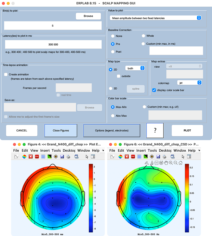
We can see this better by plotting scalp maps. Let’s start with the voltage. Select the original ERPset (with the EOG channels removed) in the ERPsets menu, and select EEGLAB > ERPLAB > Plot ERP > Plot ERP scalp maps. Set the plotting parameters as shown in Screenshot 5.3. We’re going to plot the difference wave (Bin 5), using the mean voltage from 300 to 500 ms. When everything is set, click PLOT, and you should see a scalp map like the one in the lower left of Screenshot 5.3. Note that the negative voltage is centered at the CPz electrode site and broadly distributed, with a slight bias toward the right hemisphere (which is typical for the N400).
Now select the ERPset with the current density and repeat the procedure for plotting the scalp map. The result should like the map in the lower right of Screenshot 5.3. Note that the negativity is now much sharper, and you can actually see separate foci over the left and right hemispheres. The most important thing, however, is that we are now looking at (an estimate of) the current flowing out of the scalp at each location, not a potential between each location and the reference site. The location of the original reference site no longer matters.