In a typical oddball experiment, there are two categories of stimuli, one of which is rare (called the oddballs or targets) and one of which is frequent (called the standards or nontargets). For example, you might present a sequence of Xs and Os in the middle of a video monitor, with 10% Xs and 90% Os. The Rare category will elicit a much larger P3b component than the Frequent category, but only if participants are actively discriminating between the two categories. For example, if participants are asked to judge the colors of the Xs and Os, you won’t see a larger P3 to the Rare Xs than to the Frequent Os. However, if participants are instructed to press one button for Xs and another button for Os, this requires making an active categorization of each stimulus as an X or an O, and you’ll see a much larger P3b for the Xs than for the Os. However, it’s not the motor response per se that leads to the P3b. The Xs will also produce a larger P3b than the Os if the task is to press a button for the Os and make no response for the Xs.
Researchers have known since the 1960s that the amplitude of the P3b is inversely related to the probability of the eliciting stimulus. That is, the P3b will be larger if the oddballs are 20% probable than if they are 30% probable, and the P3b will be even larger if the oddballs are 10% probable (Duncan-Johnson & Donchin, 1977). A fundamentally important but not widely appreciated fact is that it is not the probability of the physical stimulus that determines P3b amplitude, but instead the probability of what I call the task-defined category. For example, my lab once ran an oddball experiment in which 15% of the stimuli were the letter E and the other 85% were randomly selected from all the non-E letters (Vogel et al., 1998). The task was to press one button for the letter E and another button for non-E letters. The letter E was more common than any other individual letter, but the task required participants to categorize each stimulus as E or non-E, and the E category was less frequent than the non-E category. As a result, the E stimuli elicited a much larger P3b than the non-E stimuli. You can learn more about the P3b component in Chapter 3 of Luck (2014) or in John Polich’s chapter on the P3 family of components in the Oxford Handbook of ERP Components (Polich, 2012).
Many oddball experiments contain an obvious confound: If 10% of the stimuli are Xs and 90% are Os, then the Xs and Os differ both in the shape of the letter and the probability of occurrence. This probably doesn’t have much impact on the P3b component, but confounds like this are easy to avoid, so I’m always surprised that so many experiments have this confound. An easy way to solve this is to counterbalance the probabilities: Use 10% Xs and 90% Os for half the trial blocks and 90% Xs and 10% Os for the other half. This makes it possible to compare the ERP elicited by an X when it is Rare to the ERP elicited by an X when it is Frequent. And we can do the same for the Os. In other words, we can hold the stimuli constant and vary only the probability. To make things simpler, we can average the X-Rare and O-Rare ERPs together and compare the result to the average of the X-Frequent and O-Frequent ERPs. Many experiments use this approach (but not as many as I would like!).
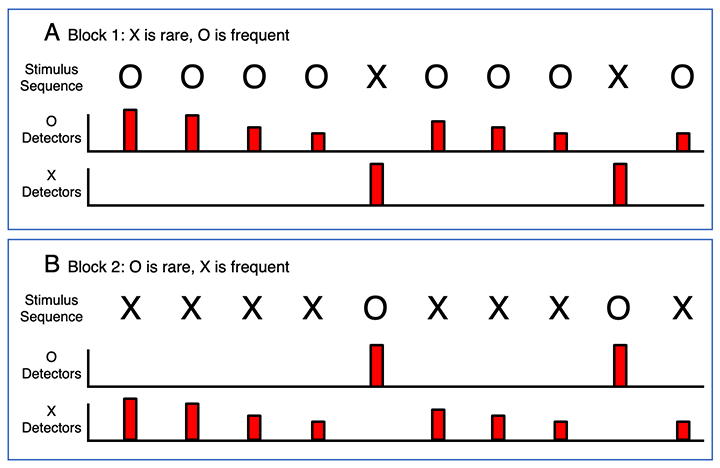
However, as illustrated in Figure 6.1, a subtle adaptation confound still remains when this counterbalancing is used. Imagine that X is Rare and O is Frequent in the first trial block, and participants press one button for the Xs and another for the Os. Neurons in visual cortex that are sensitive to the O shape will tend to become adapted by the frequent occurrence of the O stimuli, but neurons that are sensitive to the X shape will not become adapted given the infrequent occurrence of this shape. As a result, the sensory response will be smaller for the O stimuli than for the X stimuli. In the second trial block, O is Rare and X is Frequent. Now the X-sensitive neurons become more adapted than the O-sensitive neurons, and the sensory response will be smaller for the Xs than for the Os. So, even though we have counterbalanced which stimulus is Rare and which is Frequent, we still get a larger sensory response for the Rare category than for the Frequent category.
Figure 6.1. Example of the sensory adaptation confound that is present in nearly all oddball experiments. The height of each bar represents the magnitude of the sensory response to a given stimulus.
This exemplifies what I call the Hillyard Principle of experimental design: Keep the stimuli constant and vary only the psychological conditions. To follow this principle, you must keep the entire sequence constant across conditions, which we are not doing in the counterbalanced design shown in Figure 6.1. That is, we are using different sequences of stimuli to create our Rare and Frequent categories, and any differences in the ERPs for these categories could be a result of physical stimulus differences rather than the psychological categories of Rare and Frequent.
The Hillyard Principle
The Hillyard Principle is named after my PhD advisor, Steve Hillyard. When I was a grad student, we were constantly reminded to keep the stimuli constant and vary the psychological conditions (usually by varying the instructions). Steve was a master of experimental design, and he had a huge impact on the field by developing extremely rigorous designs (and instilling this ethos into his many graduate students and postdocs).
The sensory ERP components are very sensitive to small differences in stimuli, and the Hillyard Principle is especially important when you see differences between conditions at relatively short latencies (e.g., <200 ms after stimulus onset). If an experiment does not follow the Hillyard Principle, it’s usually impossible to interpret any early effects (unless, of course, the goal of the experiment was to examine the effects of stimulus manipulations on sensory activity). However, it’s a good idea to follow the Hillyard Principle even when you’re looking at later effects, because it’s difficult to be 100% certain that a late effect isn’t a consequence of an early sensory confound.
Some experimental questions are difficult to answer while following the Hillyard principle. For example, imagine that you wanted to compare the ERPs elicited by nouns and verbs (presented as auditory speech signals). You don’t have any control over what nouns and verbs sound like, and it would be difficult to create instructions that make a participant treat the word “chair” as a noun in some trial blocks and a verb in other blocks. But if you were really motivated, you could actually achieve this kind of control by using two groups of participants who spoke different languages. For example, if you compared monolingual English speakers and monolingual Mandarin speakers, you could ask whether nouns and verbs that are known by an individual produce a difference that is not present for nouns and verbs that are unknown by that individual.
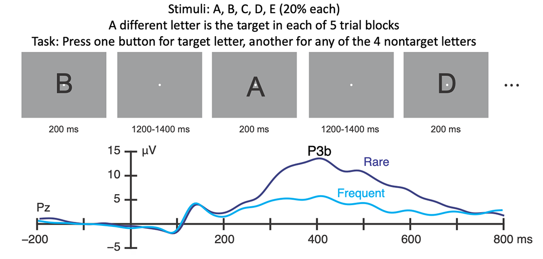
In the ERP CORE, we designed the P3b experiment to follow the Hillyard principle. As illustrated in Figure 6.2, the stimuli were the letters A, B, C, D, and E, presented in random order in the center of the video display. Each of these letters was 20% probable. Each participant received 5 trial blocks, each containing 40 trials, and a different letter was designated the target in each block. They were instructed to press one button for the target letter and another button for any of the four nontarget letters. For example, when D was designated the target, they would press one button for D and a different button for A, B, C, or E. As a result, D was in the Rare category when it was designated the target and was in the Frequent category when one of the other four letters was designated the target. Thus, we followed the Hillyard Principle: we kept the sequence of stimuli constant and varied only the task instruction.
What it Means to Keep the Sequence Constant
If we had used the same exact sequence of letters in each trial block, it is possible that participants would have learned the sequence. We therefore created a new randomized sequence for each block, but these sequences were created using the same rules and differed only randomly. That rules out any systematic differences in the physical stimuli between trial blocks.
Figure 6.2 also shows the grand average ERP waveforms for the Rare and Frequent stimulus categories (from the Pz channel, with the average of P9 and P10 as the reference). The Rare waveform contains equal numbers of trials for which A, B, C, D, and E were designated the target. The Frequent waveform also contains equal numbers of trials for which A, B, C, D, and E were designated the target. Thus, the larger P3b observed for the Rare category than for the Frequent category must reflect the Rareness of the task-defined category, not the rareness of the physical stimuli. It took a lot of thought and effort to design the experiment this way, but I really enjoy the process of designing experiments, especially when I need to come up with some kind of creative “trick” to rule out all possible confounds.
Figure 6.2. Experimental paradigm and grand average ERP waveforms from the ERP CORE visual oddball P3b experiment.