Let’s make averaged ERPs for the bins we created. We still have continuous EEG data, so we first need to divide the data into epochs, with the time-locking event code as time zero. Make sure that the correct dataset is active (12_P3_corrected_elist_bins) and select EEGLAB > ERPLAB > Extract bin-based epochs. Use the default epoch of -200 to 800 ms and the prestimulus interval as the baseline correction period. Click RUN and keep the default name of 12_P3_corrected_elist_bins_be for the new dataset. Take a look at the epoched data (using EEGLAB > Plot > Channel data (scroll)) to make sure everything looks okay. As you may recall from Chapter 2, EEGLAB plots 5 epochs on a screen by default, making the epoched data look a lot like continuous data—you need to look closely to see the boundaries between the epochs.
Once you’ve looked at the EEG epochs, select EEGLAB > ERPLAB > Compute averaged ERPs. You should be able to use the default settings and just click RUN. Name the resulting ERPset 12_P3, and save the ERPset as a file named 12_P3.erp. Now plot the ERPs (using EEGLAB > ERPLAB > Plot ERP > Plot ERP waveforms). It’s a good idea to click the RESET button in the plotting GUI to get rid of any custom settings from the last time you plotted ERPs. We only have two bins, so you can keep it set to plot all bins. You should see something like Screenshot 6.2.
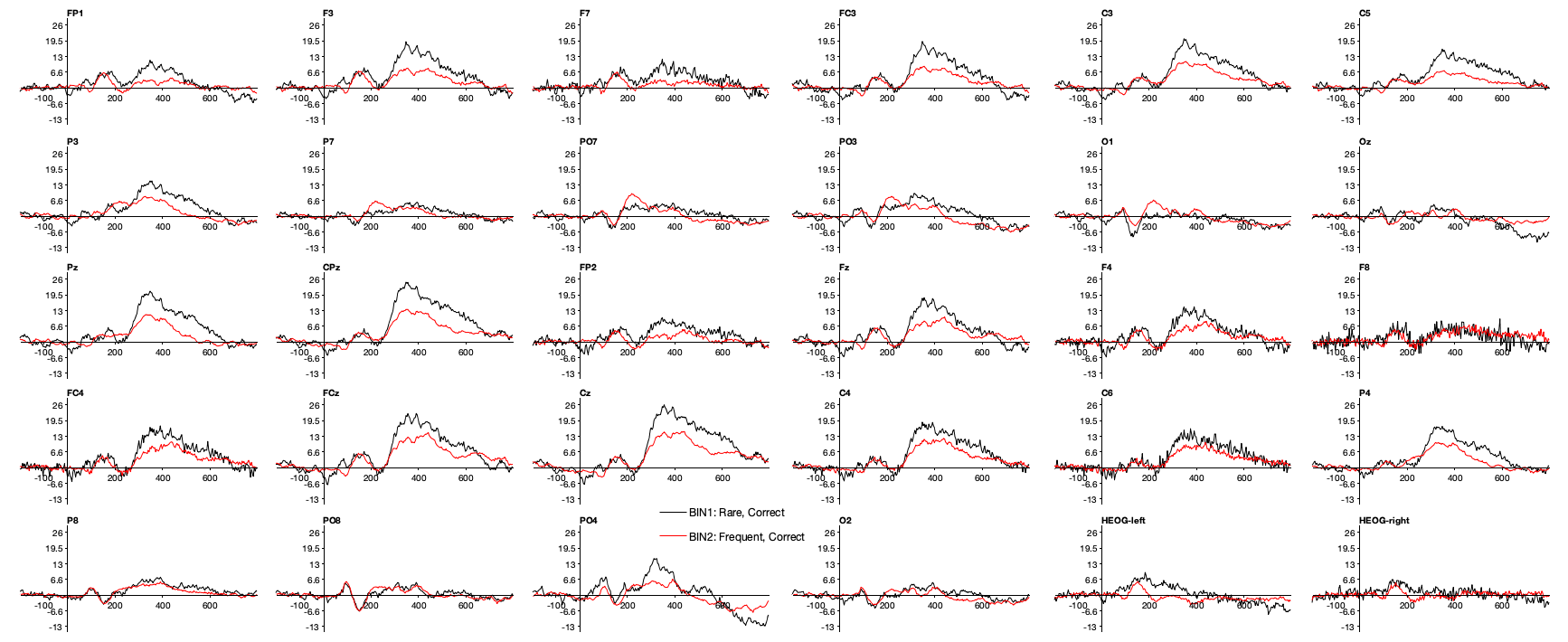
Screenshot 6.2
Compare the waveforms at Pz with the grand average waveforms shown in Figure 6.2. Pretty similar! But that’s only because I intentionally chose a participant whose ERPs looked like the grand average for the exercises in this chapter. There are tremendous individual differences in ERP waveforms (largely due to nonfunctional differences in biophysical factors like skull thickness), and the ERPs for most of the participants in this study don’t look this much like the grand average. Averaging (whether across trials or across participants) is often necessary, but the result is something of a fiction. As I like to say, “averaging hides a multitude of sins.”
Although published papers often focus on just a few electrode sites, you should always look at the whole set of channels to verify that the scalp distribution is sensible. With a reference at or near the mastoids, the P3b effect (defined as the difference between Rare and Frequent) should be biggest along the midline near Cz and Pz. This participant’s P3b is a little more frontal than is typical for a visual paradigm, and I would ordinarily expect a smaller effect at Fz and a larger effect at Oz. But given the large range of individual differences in ERPs, this participant’s data look pretty normal.
You can also see quite a bit of high-frequency noise in the lateral frontal and central channels over the right hemisphere (especially F8). The noise in F8 and surrounding channels is probably EMG from the temporalis muscle (the muscle near the temples that is used to contract the jaws). If you scroll through the original EEG data, you can also see the high-frequency noise in the single trials. My guess is that this participant was clenching their jaw just a little bit, mainly on the right side.