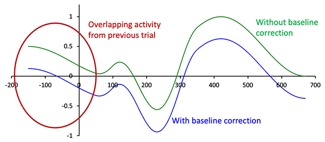
A concern often arises in a sequential analysis like the one we performed in this chapter, namely that the results are distorted by overlapping activity from the previous trial. A simple example of overlap is shown in Figure 6.3, which simulates an experiment in which a stimulus is presented every 700 ms. The falling edge of the P3b from one trial is present during the prestimulus baseline period of the next trial, which impacts the baseline correction procedure. That is, baseline correction involves taking the mean voltage during the baseline period and subtracting it from each point in the waveform. The positive voltage from the overlap in the baseline causes us to overestimate the true baseline voltage, and the entire waveform is shifted downward as a result. You might think that we should just skip the baseline correction step, but it’s essential in 99.9% of experiments because there are huge sources of low-frequency noise that would contaminate the waveform if we did not subtract the baseline.
Figure 6.3. Example of the impact of overlap on an ERP waveform before and after baseline correction. In this example, we are assuming that a stimulus is presented every 700 ms, so the falling edge of the P3b from one trial is present during the prestimulus period of the next trial. When this positive voltage is subtracted out by the baseline correction process, it shifts the poststimulus waveform downward.
Some amount of overlap is present in most experiments, but it’s not usually a problem unless it differs across conditions. For example, if the P3b on the previous trial was larger in Condition A than in Condition B, this would produce a larger positive voltage in the baseline of Condition A. The baseline correction procedure would then push the rest of the waveform farther downward in Condition A than in Condition B. As a result, the differences in overlap between Conditions A and B during the prestimulus period end up creating a difference between the waveforms for these conditions in the poststimulus period. This is a fundamentally important issue, and I recommend reading Marty Woldorff’s foundational paper on overlapping ERP activity (Woldorff, 1993). In fact, it’s on my list of papers that every new ERP researcher should read.
I hope you can now see why I’m a little worried about comparing the Rare-preceded-by-Rare waveform with the Rare-preceded-by-Frequent waveform. The overlapping voltage in the baseline might be larger when the previous trial was Rare (yielding a large P3b) than when it was Frequent. The baseline correction procedure would then push the waveform farther downward on Rare-preceded-by-Rare trials than on Rare-preceded-by-Frequent trials, artificially creating the appearance of a smaller (less positive) P3b in the Rare-preceded-by-Rare waveform than in the Rare-preceded-by-Frequent waveform.
However, if the time between trials is long enough, the P3b from the previous trial will have faded prior to the baseline period of the current trial. In the ERP CORE visual oddball P3b experiment, the time from one stimulus onset to the next (the stimulus onset asynchrony or SOA) was 1400-1600 ms. The 200-ms prestimulus interval that we’ve used for the current trial therefore began at least 1200 ms after the onset of the stimulus from the previous trial. That seems like it ought to be enough time for the P3b from the previous trial to end, but it’s difficult to be certain without additional analyses.
In this exercise, we’re going to repeat the sequential analysis from the previous exercise, but taking a closer look at the overlapping activity from the previous trial. In particular, we’re going to dramatically increase the length of the prestimulus portion of the epoch so that we can see the previous-trial ERP as well as the current-trial ERP. And we’re going to see what happens when we use different parts of the prestimulus period for baseline correction.
We’re simply going to change the epoch length, so we can start with the EEG dataset you created using BINLISTER in the previous exercise, named 12_P3_corrected_elist_bins_seq. Make it the active dataset (which may require loading it from the file you saved in the previous exercise). Now epoch the data (EEGLAB > ERPLAB > Extract bin-based epochs) using an epoch time range of -1800 800 and a baseline correction period of -1800 -1600. If you look at Figure 6.2, you’ll see that the maximum SOA is 1600 ms, so the period from -1800 to -1600 ms is always prior to the previous trial. By using this as our baseline, we can be certain that the baseline correction won’t be influenced by whether the previous trial was the Rare or Frequent category.
Now average the data, naming the ERPset 12_Sequential_LongBaseline and saving it as a file named 12_Sequential_LongBaseline.erp. Plot the ERPs from Bins 1 and 2, but specify None in the Baseline Correction area of the plotting GUI so that it doesn’t re-baseline the data. (Alternatively, you could specify Custom with a time range of -1800 -1600).
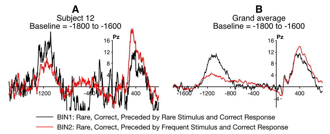
Screenshot 6.7A shows what it should look like in the Pz channel. You can still see that the current-trial P3b is larger for Rare-preceded-by-Frequent than for Rare-preceded-by-Rare. That suggests that the sequential effect was saw before was not a result of the combination of overlap and baseline correction. However, the data are pretty noisy, so I ran this analysis on all the participants. The grand average in Screenshot 6.7B confirms that the sequential effect remains when the data are baselined relative to the prestimulus period from the previous trial.
The grand average waveforms also make it clear that differential overlap is a real concern. That is, the persisting voltages from the previous trial were somewhat different according to whether that trial was Rare or Frequent, potentially contaminating the baseline period from the current trial. However, the overlapping activity seems to go in the opposite direction of the sequential effect, being more negative (near time zero) when the previous trial was Frequent than when it was Rare, whereas the current-trial P3b was more positive.
Screenshot 6.7
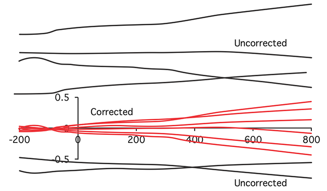
Although the grand averages looked fine when we used the prestimulus period from the prior trial as the baseline interval, this approach can decrease the precision and reliability of the ERP waveforms. As illustrated in Figure 6.4, this decline in precision occurs because the single-trial EEG voltage tends to drift gradually over time in a random direction, and the trial-to-trial variability increases as you get farther away from the baseline period. This increased variability increases the error in measuring the “true” amplitude, increasing variability across participants and thereby decreasing statistical power. Indeed, the waveforms in some of the channels look pretty crazy with this distant baseline.
Figure 6.4. Illustration of the combined effects of low-frequency drift and baseline correction. The EEG is superimposed on low-frequency signals (mainly arising from the skin) that drift slowly over time in a random direction. When the data are baseline-corrected, this forces the voltages to be similar during the baseline period, but the voltage tends to drift farther away from the baseline value, causing a gradual increase in trial-to-trial variability over time.
You can use the Standardized Measurement Error to quantify this increase in measurement error. Take a look at the aSME values for the Pz channel in Bin 1 (EEGLAB > ERPLAB > Data Quality options > Show Data Quality measures in a table). We’ll want to compare these values to the corresponding values from the original sequential analysis in which the baseline correction period was -200 to 0 ms. (To save the current aSME values, you can either copy them from the table and paste them in a word processor or save the values in a spreadsheet by clicking the button for Export these values, writing to: Excel.) Load the ERPset you saved previously as 12_P3_Sequential.erp and look at the aSME values in that dataset, which was baselined from -200 to 0.
How do the aSME values differ between the data with the two different baseline periods? You should see that they are substantially worse (larger) when the -1800 to -1600 period was used as the baseline. That’s exactly what we’d expect from Figure 6.4. So, although using a distant time period for baseline correction can sometimes be valuable for assessing overlap, it comes at the cost of increased measurement error. As a result, I find that analyses like these are mainly useful descriptively and not for statistical analysis. In other words, it’s usually enough to look at the grand averages and see that the effects are largely the same with the two different baseline periods without performing a statistical analysis on the data with the distant baseline period.