It’s now time to see how artifact detection works in actual data. We’ll start by detecting blinks, which are big and easy to detect. We’ll begin with the most common blink detection algorithm, which simply asks whether the voltage falls outside a specified range at any point in the epoch for a given channel. This is a pretty primitive algorithm, and the next exercise will show you a much better approach.
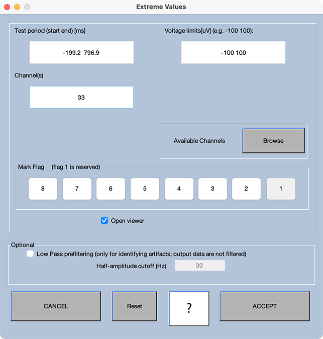
Start by loading the data from Subject #1 in the MMN experiment, which is in the file named 1_MMN_preprocessed_interp. This is the same dataset that we examined in the previous chapter, after the C5 channel was interpolated. Artifact detection operates on epoched data, so select EEGLAB > ERPLAB > Extract bin-based epochs, using an epoch of -200 to 800 ms and Pre as the baseline. Name the resulting dataset 1_MMN_preprocessed_interp_be. Now select EEGLAB > ERPLAB > Artifact detection in epoched data > Simple voltage thresholds and set the parameters as shown in Screenshot 8.1. In particular, specify 33 as the Channel (this is the VEOG-bipolar channel) and voltage limits of -100 100. These voltage limits indicate that an epoch should be flagged for rejection if the voltage is more negative than -100 µV or more positive than +100 µV at any time in this channel. Blinks will be largest in the VEOG-bipolar channel, so there’s no point in looking for blinks in other channels. We’ll worry about other types of artifacts later.
You might wonder why the default Test period is set to -199.2 796.9 rather than -200 800 (which is what you specified for the epoch). The answer is that the data were originally sampled at 1024 Hz and were then downsampled to 256 Hz for the analyses provided in the ERP CORE paper. As a result, we have a sample every 3.90625 ms, and we don’t have samples at exactly -200 and +800 ms. In the previous chapters, I downsampled to 200 Hz instead, yielding a sample every 5 ms. But I thought it was time for you to see what happens when the sampling period isn’t a nice round number.
Don’t worry about the flags; I’ll discuss them later. Click ACCEPT to apply the algorithm to the selected dataset.
Screenshot 8.1
Once the algorithm has finished, you will see two windows. One is the standard window for saving the updated dataset. The other is the standard window for plotting EEG waveforms. The idea is that you’ll use the plotting window to make verify that the artifact detection worked as desired. If so, you’ll use the other window to save the dataset. If you’re not satisfied with which epochs were flagged, you’ll click Cancel and try again with new artifact detection parameters.
However, before you start scrolling through the plotting window, it’s important to see how many artifacts were detected. This information is shown in the Matlab command window. You can see the number and percentage of epochs in which artifacts were detected in each bin and the total across bins. In most cases, I mainly worry about the total (because the percentage is much more meaningful when based on a large number of trials). You can see that 17.8% of epochs were rejected. That’s reasonable. As noted above, my lab always throws out any participants for whom more than 25% of epochs were rejected, so this participant would be retained.
Now let’s scroll through the EEG data and see how well the algorithm performed at flagging epochs with blinks and not flagging epochs without blinks. I recommend setting the vertical scale to 100. Keep in mind that we’re now looking at epochs rather than continuous data, and the plotting window shows 5 epochs per screen by default. (If you have a large screen, I recommend going to Settings > Time range to display in the plotting window and telling it to show 10 or even 15 epochs per screen.) Epochs that have been flagged for artifacts are highlighted in yellow. Recall that Subject #1 had beautiful EEG in the beginning of the session, so you won’t see any flagged epochs at first. But you still need to make sure that there aren’t any blinks that weren’t detected, so scroll through the epochs and look at the VEOG and Fp1/Fp2 channels to make sure that everything looks okay.
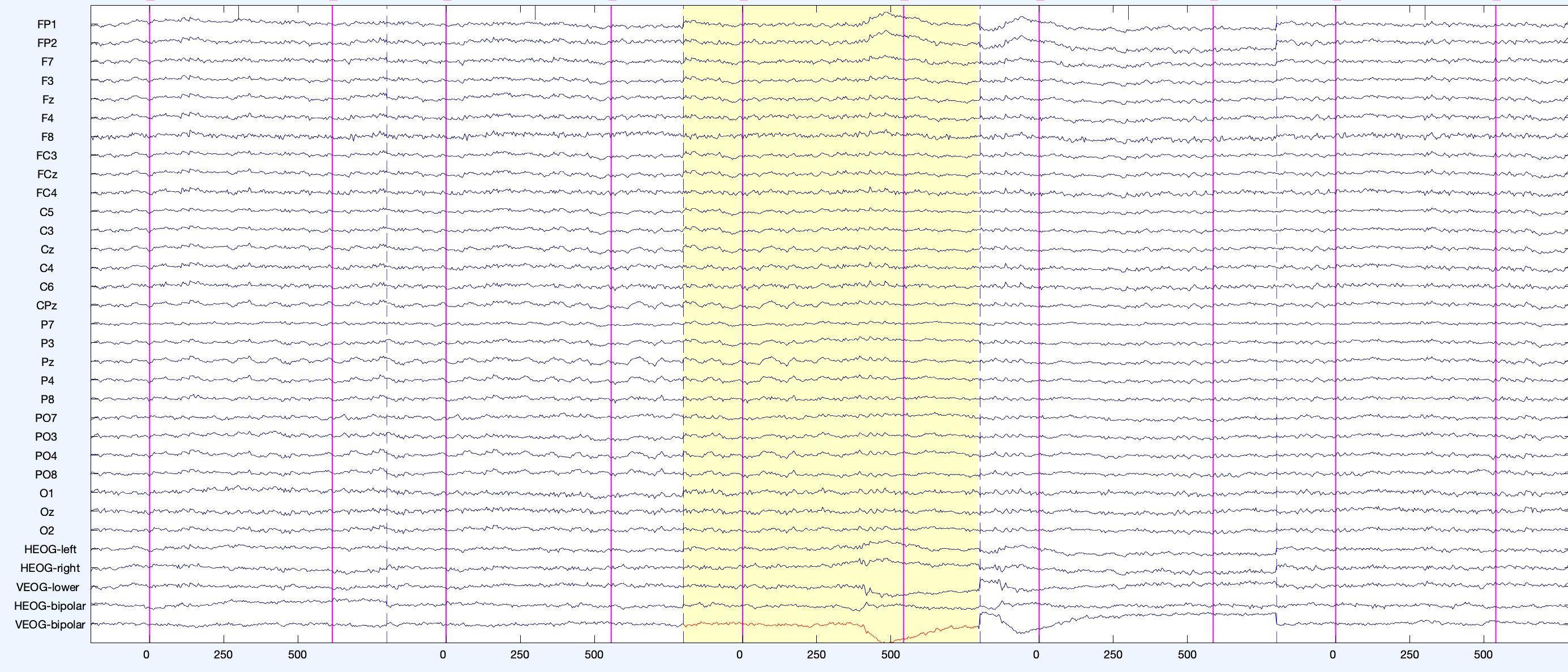
Epoch 103 should be the first marked epoch (see Screenshot 8.2). The waveform for the offending channel is drawn in red. You can see a classic blink shape and scalp distribution. Success!
But this is immediately followed by a failure in Epoch 104. Because we have a stimulus every 500 ms, but each epoch lasts for 1000 ms, the initial part of one epoch is the same as the latter part of the previous epoch. So, the blink that peaked just before 500 ms in Epoch 103 appears just before time zero in Epoch 104. Because the blink is during the baseline in Epoch 104, the baseline correction procedure reduced the maximum voltage during the epoch, and the blink is not detected.
Screenshot 8.2
Keep scrolling. You’ll notice a large muscle burst in Epoch 107 that isn’t flagged. But that’s OK—we’re looking for blinks right now, and we’ll test for other artifacts later. You’ll also see a blink that appears in the poststimulus period of Epoch 121 and in the prestimulus period of Epoch 122. This blink was larger than the one in Epochs 103 and 104, and the blink was successfully detected in both Epochs 121 and 122. The blink appearing in Epochs 162 and 163 was also successfully detected. However, the blink that appears in Epochs 169 and 170 was missed in Epoch 170.
If you keep scrolling, you’ll also see that high-frequency noise (almost certainly EMG) caused Epoch 463 to be flagged. You can tell that there was no blink in this epoch because there was no positive-going voltage in Fp1 and Fp2, just a small negative-going voltage in VEOG-lower combined with some high-frequency noise. There is no reason to reject this epoch: The voltages in VEOG-lower are very localized and unlikely to impact our scalp EEG recordings. Epochs 525 and 526 are also unnecessarily flagged for rejection. In these epochs, a combination of a slow, non-blink-like voltage deflection and high-frequency noise in Fp2 (but without an opposite-polarity deflection in VEOG-lower) produced a large enough voltage in VEOG-bipolar for the voltage to exceed our ±100 µV threshold.
You can now close the plotting window and save the dataset that was created, naming it 1_MMN_preprocessed_interp_be_ar100. We’ll need it for a later exercise.