To decide on the threshold for rejecting trials with eye movements, we need to return to our goals for artifact rejection. What threshold maximizes our data quality while avoiding confounds in our data?
Let’s first consider whether horizontal eye movements are a confound in this experiment. Specifically, might horizontal eye movements cause different voltages at our FCz electrode site on deviant trials relative to standard trials? This is unlikely for two reasons. First, because FCz is on the midline, it should be near the line of zero voltage between the positive and negative sides of the voltage field produced by horizontal eye movements. Second, there is no reason to suspect that the frequency of leftward versus rightward eye movements would differ between deviants and standards. However, this is just an assumption, and we should check to make sure.
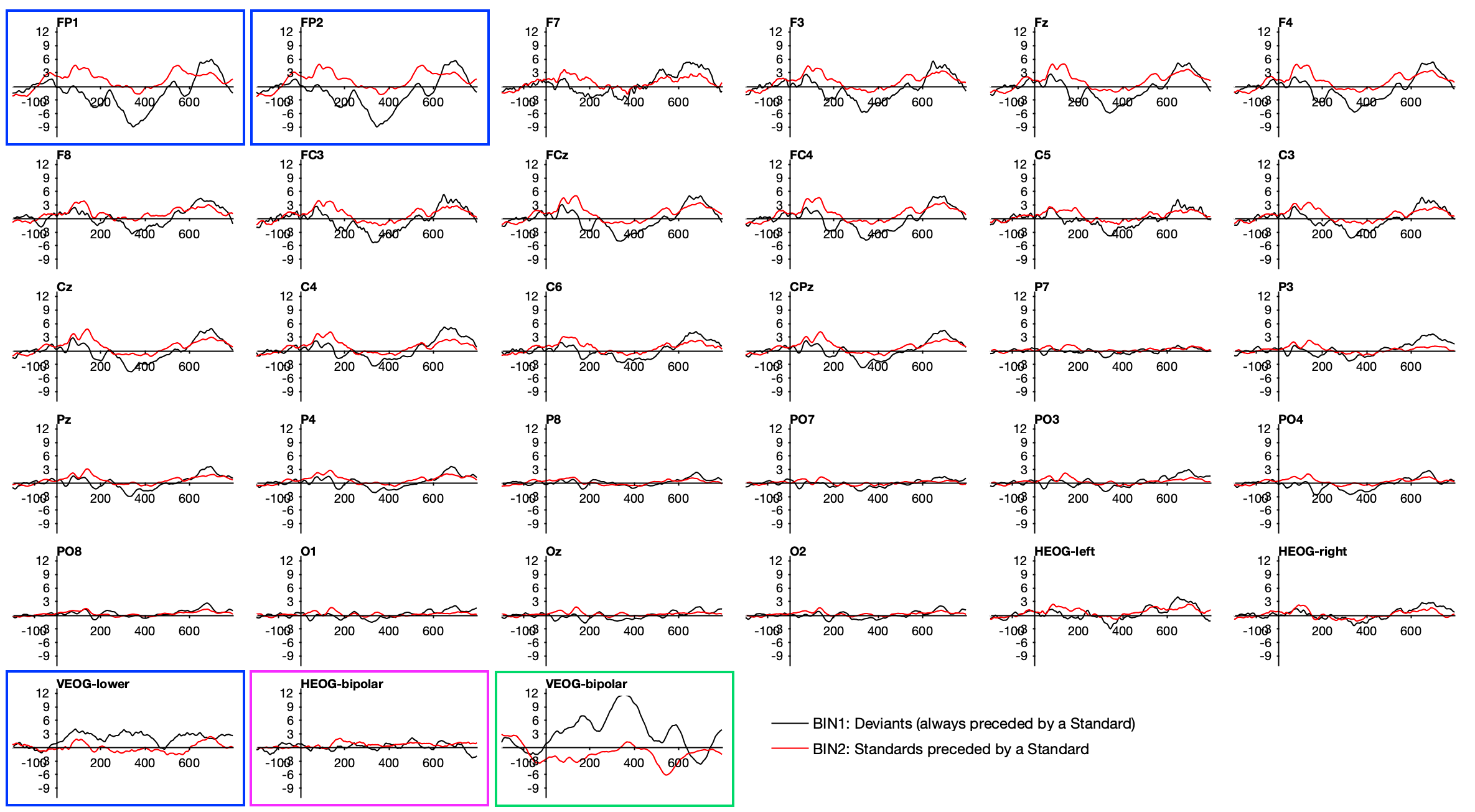
We can assess this assumption by looking at the ERP waveforms without any artifact rejection. To do this, select the dataset for Subject 10 that was created prior to any artifact detection (10_MMN_preprocessed_filt_be) and then select EEGLAB > ERPLAB > Compute averaged ERPs. If you plot the resulting ERP waveforms, you’ll see a large voltage deflection for the deviants in the VEOG-bipolar channel (indicated by the green box in Screenshot 8.6). You can also see that this voltage is opposite in polarity below the eyes (VEOG-lower) versus above the eyes (Fp1 and Fp2; see the blue boxes in Screenshot 8.6). This indicates that this participant blinked more following the deviants than following the standards, just as we saw for Subject 1 (see Figure 8.2.A). However, unlike Subject 1, Subject 10 showed this pattern even during the MMN time window, so blinks could confound the MMN effects for this participant.
Screenshot 8.6
Now look at the HEOG-bipolar channel (indicated by the magenta box in Screenshot 8.6). The differences between deviants and standards in that channel are not any larger than the noise deflections in the prestimulus baseline period. This tells us that we don’t have to worry about differences between deviants and standards in the frequency of leftward versus rightward eye movements, confirming our assumption. This means that we mainly need to be concerned about whether the eye movements are a source of noise, not a confound.
To assess noise, we can ask how the artifact rejection impacted the SME values. Specifically, we’ll look at the SME values after rejecting only trials containing blinks, rejecting trials with blinks and eye movements using a 32 µV eye movement threshold, and rejecting trials with blinks and eye movements using a 16 µV eye movement threshold.
To start, let’s get the SME values after rejecting trials with blinks but before rejecting trials with eye movements. Make the dataset named 10_MMN_preprocessed_filt_be_noblinks active, and EEGLAB > ERPLAB > Compute data quality metrics (without averaging). In the Data Quality section of the GUI, select Custom parameters, click the Set DQ options… button, and create a custom time range of 125-225 ms. Make sure that the main GUI is set to exclude epochs marked during artifact detection, and then click RUN. In the data quality table that appears, look at the aSME values for Bin 1 and Bin 2 from the FCz channel in the 125-225 ms time range. These values will be our reference points for asking whether rejecting trials with eye movements makes the data quality better (because of less random variation in voltage) or worse (because of a reduction in the number of epochs being averaged together). Keep the data quality window open so that you can refer to it later.
Now repeat this process with the datasets in which eye movements were flagged for rejection using a threshold of 32 µV (10_MMN_preprocessed_filt_be_noblinks_HEOG32) and 16 µV (10_MMN_preprocessed_filt_be_noblinks_HEOG16). Compare the resulting data quality tables with the data quality table you obtained without rejection, focusing on the aSME values for Bin 1 and Bin 2 from the FCz channel in the 125-225 ms time range.
These values are summarized in Table 8.1. You can see that the data quality was slightly reduced (i.e., the aSME was increased) when large eye movements were rejected by means of the 32 µV threshold and substantially reduced when virtually all eye movements were rejected by means of the 16 µV threshold. Given that the previous analyses indicated that horizontal eye movements were not a confound, the 16 µV threshold appears to be taking us farther from the truth rather than closer to the truth (because it impairs our ability to precisely measure MMN amplitude). The 32 µV threshold decreases the data quality only slightly (probably because there is some benefit of reduced noise but some cost of a smaller number of trials). I would be inclined to go with this 32 µV threshold (instead of not excluding trials with horizontal eye movements), even though it slightly reduces the data quality, just in case there is some small confounding effect of large eye movements that wasn’t obvious.
Table 8.1. Effects of eye movement rejection on data quality and percentage of rejected trials.
Rejection
aSME for Deviants
aSME for Standards
% Rejected
Blinks Only
0. 8264
0.5353
31.8%
Blinks + Eye Movements (32 µV)
0. 8335
0.5874
41.5%
Blinks + Eye Movements (16 µV)
0.9901
0.7437
67.6%
Viewing a Summary of Artifacts
Table 1 shows the percentage of rejected trials. This information was printed to the Matlab Command Window when the data quality metrics were computed (and are also printed when you average). If you want to see this information for a given dataset at a later time, select the relevant dataset and then select EEGLAB > ERPLAB > Summarize artifact detection > Summarize EEG artifacts in a table. You’ll then be asked where you want to save the summary. I usually choose Show at Command Window.
As you have seen, there is some subjectivity involved with artifact rejection. In my experience, a well-trained researcher can meaningfully increase the final data quality and avoid confounds by carefully setting the artifact detection parameters individually for each participant in this manner. It takes some time, but you will get much faster as you gain experience. The two participants we’ve examined so far in this chapter are particularly challenging cases that require some careful thought and analysis, but most of the participants in this study were much more straightforward. I find that we can use a standard set of detection parameters in about 80% of participants in my lab’s basic science experiments, and it takes only 5–10 minutes to verify that everything is working fine in these participants.
Beyond the time investment, it’s also important to consider whether customizing the artifact rejection for each participant might lead to some kind of bias in the results. Most basic science ERP studies involve within-subjects manipulations, in which the same artifact detection parameters are used for all conditions for a given participant. Because the parameters are identical across conditions, there is little opportunity for bias. In theory, the experimenter could try many different artifact detection parameters for a given participant and then choose the parameters that produce the desired effect. But this is obviously cheating. If someone wants to cheat, there are much easier ways to do it, so I don’t worry much about this possibility. To avoid unconscious bias, you should avoid looking at the experimental effects in the averaged ERP waveforms when you’re setting the parameters (although you may need to look at the averaged EOG waveforms to assess the presence of systematic differences in artifacts between conditions).
My advice is different for research that focuses on comparing different groups of participants (e.g., a patient group and a control group). In these studies, the main comparisons are between participants, and now we may have different artifact detection parameters for our different groups. This could lead to unintentional biases in the results. To minimize any biases, I recommend that the person setting the artifact detection parameters for the individual participants should be blind to group membership. For example, in my lab’s research on schizophrenia, the person setting the artifact detection parameters is blind to whether a given participant is in the schizophrenia group or the control groups. That’s a bit of a pain, but it’s worth it to avoid biasing the results. Note that some subjectivity also arises in artifact correction (e.g., choosing which ICA components to eliminate), so the person doing the correction should also be blind to group membership.
When to set artifact detection parameters (and how to avoid a catastrophe)
Imagine that you spend 9 months collecting data for an ERP study, and at the end you realized that there was a major problem with the data that prevented you from answering the question that the study was designed to answer. Your heart would start racing. Your face would become flushed. You would feel like vomiting. And you would want to crawl into a hole and never come out.
Would you like to avoid that situation? If so, then here’s an important piece of advice: Do the initial processing of each participant’s data within 48 hours of the recording session. This includes every step through averaging the data and examining the averaged ERPs. Of course, this includes setting the artifact detection parameters. And it includes quantifying the behavioral effects (which is the step that people most frequently forget).
If you don’t do this, there is a very good chance that there will be a problem with your event codes, or with artifacts, or with something unique to your experiment that I can’t anticipate, and that this problem will make it impossible for you to analyze your data at the end of the study. I have seen this happen many, many, many times. Many times!
You can catch a lot of these problems by doing a thorough analysis of the first participant’s data before you run any additional participants. And in my lab, we have a firm rule that experimenters aren’t even allowed to schedule the second participant until we’ve done a full analysis of the first participant’s data. I estimate that we catch a problem about 80% of the time when we analyze the first participant’s data. So you absolutely must do this.
However, some problems don’t become apparent until the 5th or the 15th participant. And sometimes a new problem arises midway through the study. For this reason, you really must analyze the data from each participant within a couple days.
There is another side benefit to this: You won’t be in the position of needing to set the parameters for 30 participants in a single two-day marathon preprocessing session. Not only would these be two of the most dreariest days of your life, it would be difficult for you to pay close attention and do a good job of setting the parameters. The task of setting the parameters is best distributed over time.