9.2: Exercise- A First Pass at ICA-Based Blink Correction

I find that it’s easiest to understand ICA by starting with an example and then explaining how it works after you’ve seen it in action. We’re going to start with the data Subject 10 from the ERP CORE MMN experiment, which we looked at in the previous chapter in the section on eye movement detection.

Launch EEGLAB (or quit and restart it if was already running). Set Chapter_9 to be Matlab’s current folder, and load the dataset named 10_MMN_preprocessed.set. Make sure you’re getting the data from the Chapter_9 folder rather than the Chapter_8 folder, because the data are preprocessed a little differently but the filenames are the same.

The dataset you loaded has been high-pass filtered at 0.1 Hz and referenced to the average of P9 and P10 (except for the VEOG-bipolar and HEOG-bipolar channels). Take a look at the data to remind yourself what it looks like. You’ll see lots of blinks and eye movements prior to the start of the stimuli at ~25 seconds.

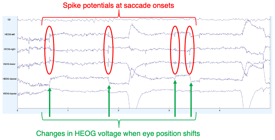
When we looked at this participant’s data in the previous chapter, the EEG had been low-pass filtered. Without the low-pass filtering, you can now more easily see the spike potential at the beginning of each eye movement, which is a result of the muscle activity that sets the eyes in motion. This is illustrated in Figure 9.1, which shows the first 5 seconds of data from Subject 10. You can see a brief spike in several channels at the moment when the HEOG voltage starts to change from one level to another (which indicates a change in gaze location from one location to another). You may want to adjust the vertical scale and number of channels being displayed so that you can see these voltage changes more clearly.

Figure 9.1 Examples of spike potentials and HEOG voltage associated with saccadic eye movements.

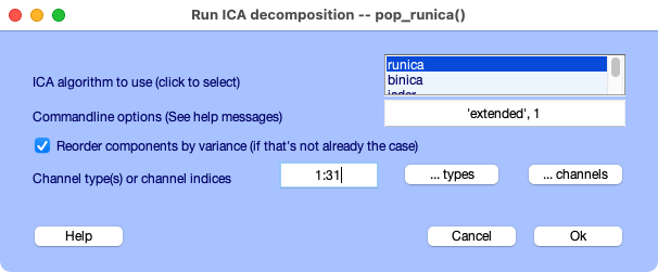
Once you’re done scanning through the EEG to see what the whole session looks like, select EEGLAB > Tools > Decompose data by ICA and set the parameters as shown in Screenshot 9.1 Everything is probably already set correctly, except for the channels, which you should set to 1:31. With this channel list, we’re including all the channels that have the same reference, and we’re excluding VEOG-bipolar and HEOG-bipolar. ICA assumes that the channels are linearly independent of each other, and the VEOG-bipolar and HEOG-bipolar were created by recombining other channels, so they would violate this assumption. However, they are useful channels to have so that we can tell when blinks and eye movements occurred even after we’ve corrected the EEG data.

 

Screenshot 9.1

Click OK to start the process of computing the ICA weights. You’ll see some text appear in the Matlab command window, followed by a long series of lines that look like this:

step 1 - lrate 0.001000, wchange 16.88431280, angledelta  0.0 deg

step 2 - lrate 0.001000, wchange 0.90426626, angledelta  0.0 deg

ICA works by training a machine learning algorithm (much like a neural network), and it can take the algorithm a very long time to converge on a solution. The amount of time depends on the number of channels, the noise level of the data, and the speed of your computer. It took over 5 minutes to reach a solution for this dataset on my laptop. If you don’t want to wait for it to finish, you can kill the process by clicking the Interrupt button that should be visible while ICA is running. If that doesn’t work, you can usually kill a Matlab process by typing Ctrl-C.

If you waited for it to finish, you should change the name of your dataset to indicate that ICA weights have been added to it. You can do this with EEGLAB > Edit > Dataset info. You can just add _rawICAweights to the name of the dataset and click OK. If you didn’t wait for the process to finish, you can just load the dataset named 10_MMN_preprocessed_rawICAweights.set, which has the ICA weights that I got when I ran the decomposition.

An easy way to see that the ICA weights have been added is to type EEG in the Matlab command window. It will show you the contents of the current EEG structure, and you can see that the fields beginning with ica are now filled:

              icaact: [31×157184 single]

             icawinv: [31×31 double]

           icasphere: [31×31 double]

          icaweights: [31×31 double]

         icachansind: [1×31 double]

ICA decomposes the EEG data into a set of independent components or ICs. These are statistically defined components, not necessarily ERP components, and they may not be biologically meaningful. I will refer to them as ICs rather than as components to maintain this important distinction.

Each IC is a spatial filter. When we apply an IC to the distribution of voltages over the scalp at a given moment in time, the output is the magnitude of that IC at that moment in time. Conveniently, ICA creates scalp maps of the ICs showing how each channel is weighted by the IC. Take a look at the scalp maps now by selecting EEGLAB > Tools > Inspect/label components by map. (You can also view the maps with EEGLAB > Plot > Component Maps). You should see something like Screenshot 9.2.

Screenshot 9.2

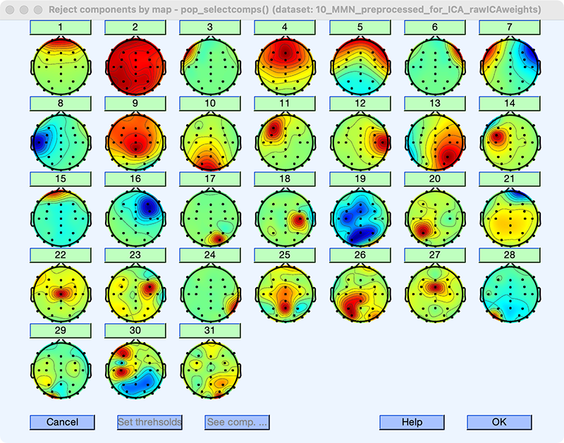
If you didn’t let the component decomposition process finish but instead loaded the file that already had the weights in it, the scalp maps you see should look exactly like those in the screenshot. However, if you ran the component decomposition process yourself, the maps might look a little different. This is because the ICA machine learning algorithm contains some randomization and therefore doesn’t yield exactly the same results every time. If things are working well, then the results should be similar if you repeat the decomposition process multiple times. If you get very different results, then something is wrong (usually either very noisy data, not enough data, or a linear dependency among your channels).

There are some things that may differ across repetitions that don’t indicate a problem. First, the ordering of the ICs might change a little. For example, the scalp maps for ICs 13 and 14 might be swapped in your data. Second, there might be small changes in the weights for a given scalp map. Third, the polarity of the scalp maps might be inverted (which we will discuss in more detail later). These are normal and no cause for concern. However, if you see radically different maps, then something is wrong.

Notice that there are 31 ICs. This is because we gave the algorithm data from 31 channels. Ordinarily, the number of ICs is equal to the number of channels. This is necessary to make the math work. But it indicates an important way in which ICA is an imperfect method for identifying the true components underlying your data. The number of channels that you record from determines the number of ICs, but putting more or fewer electrodes on the scalp doesn’t change the number of sources of brain activity!

When the decomposition algorithm finishes, it reorders the components in terms of the amount of variance in the data they account for, with IC 1 accounting for the greatest variance. If the participant blinked frequently, the IC corresponding to the blinks is usually in the top five ICs (and often IC 1). In our current example, IC 1 has the kind of far frontal scalp distribution that you’d expect for a blink. But is this really a blink IC, or is it some other kind of artifact, or maybe even frontally distributed brain activity?

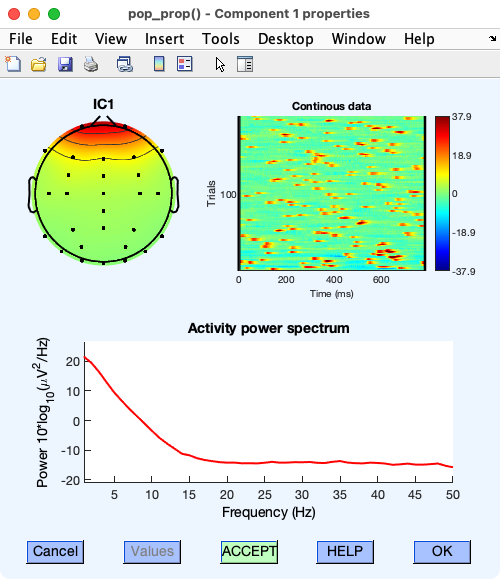
There are a few things we can check to determine whether IC 1 reflects blinks. If you click the number above IC 1, a new window will pop up showing you more details about this IC. In the upper right of the window, you’ll see a heat map showing how the magnitude of this IC varies over time. The X axis is time within a “trial” (which are arbitrary time periods when continuous data are used). The Y axis is time over the course of the recording. It’s labeled Trials but actually corresponds to time in continuous data. You can see many small red blobs. Each of those is a brief time period in which the magnitude of IC 1 was large. This is exactly what we’d expect for blinks: many brief blips of voltage. The window also shows the frequency spectrum. The spectrum for IC 1 shows a gradual decline as the frequency increases, which is also characteristic of blinks (but is also seen for many types of non-blink activity).

Screenshot 9.3

The next thing you can do (which I find the most informative) is to directly compare the time course of IC 1 with the time course of the EEG and EOG signals. Start by selecting EEGLAB > Plot > Channel data (scroll) to show the time course of the EEG and EOG signals. While that window is still open, select EEGLAB > Plot > Component activations (scroll). Then arrange the windows above and below each other as shown in Screenshot 9.4 (which is set to show 10 seconds per screen). Now you can look at how IC 1 activation varies over time and compare it to the EOG and EEG signals at the corresponding time points. Try scrolling through both windows to see whether IC 1 corresponds to the VEOG-bipolar signal. You may want to display only ~6 channels in each plotting window so that you can see these signals better.

Screenshot 9.4

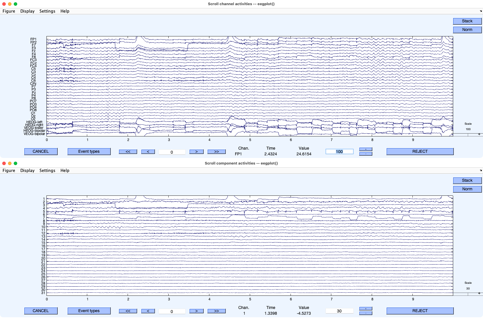
The first thing to notice is that each blink that you can see in the VEOG-bipolar channel is accompanied by a deflection with the same shape in IC 1 (e.g., at 2.2 and 4.4 seconds). You should also notice that there are occasional step-like deflections in both VEOG-bipolar and IC 1. These are vertical eye movements. Often, but not always, blinks and vertical eye movements will be captured by the same IC. Given the scalp distribution of IC 1 and its close correspondence in time with the blinks and eye movements in the VEOG-bipolar channel, we can be quite sure that this IC reflects vertical EOG activity.

Now let’s remove IC 1 from the EEG/EOG data to eliminate the blinks and vertical eye movements. Ordinarily, we would also remove other artifact-related ICs at this point (e.g., horizontal eye movements), but we’ll just focus on blinks and vertical eye movements for now. To do this, select EEGLAB > Tools > Remove components from data, put 1 in the window labeled List of component(s) to remove from data so that we remove activity corresponding to IC 1, and click OK. You’ll then see a confirmation window. Click the button in this window for plotting single trials. You should see something like Screenshot 9.5 (but I’ve told it to display the top 10 channels and show a 10-second time period). The blue waveform shows the original data and the red waveform shows what the data will look like after removing IC 1.

Screenshot 9.5

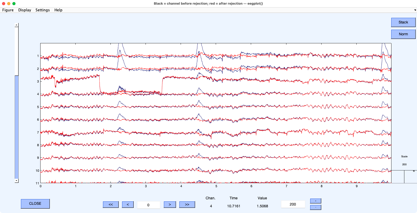
You can see that the algorithm has done a good job of eliminating the blinks and vertical eye movements. For example, the blinks at 2.2 and 4.4 seconds are now gone, and there is no longer a sudden step in voltage at 5.7 seconds. There are also some slower differences between the corrected and uncorrected data, which probably represent sustained changes in the vertical EOG corresponding to changes in eye or eyelid position.

Now click the ACCEPT button in the confirmation window, and use 10_MMN_preprocessed_rawICAweight_pruned as the dataset name. Next, plot the new dataset with EEGLAB > Plot > Channel data (scroll). You’ll see that the blinks are now gone from all channels, except for the VEOG-bipolar and HEOG-bipolar channels. We excluded those channels from ICA, and now we can use them to see when the blinks were in the original data. You can still see blinks at 2.2 and 4.4 seconds in the VEOG-bipolar channel, but the blink activity has been removed from the other channels.

If you think about it, this is something of a miracle. We’ve mathematically eliminated the contribution of blinks and vertical eye movements to the EEG at every single time point. But did this help us address the three types of problems caused by artifacts that were discussed in Chapter 8? The next exercise shows how to answer this question.