9.8: Exercise- Deleting C.R.A.P. Prior to ICA

In this exercise, we’re going to look at another type of large, idiosyncratic voltage deflection that should be eliminated prior to the ICA decomposition, namely huge C.R.A.P. In particular, we want to get rid of voltage deflections that are sufficiently large to impact the quality of the ICA decomposition but are sufficiently infrequent or irregular in their scalp distribution that they can’t be well captured by a single IC.

The participant we’ve been working with so far, Subject 10, doesn’t really have any huge C.R.A.P., so we’re going to look at Subject 6 for this exercise. Quit and restart EEGLAB, and the open the 6_MMN_preprocessed_filt_100Hz_del dataset. This dataset has already been preprocessed to improve the ICA decomposition, including filtering from 1-30 Hz, resampling at 100 Hz, and deletion of the break periods.

As usual, you should start by scrolling through the data to see what kinds of artifacts are present. In addition to the usual blinks and eye movements, you’ll see some odd-looking voltage deflections at several time points, including 70, 72, 96, 254, 403, and 413 seconds. These deflections are somewhat like blinks, but much larger and with a different and variable scalp distribution. For example, the deflection at ~70 seconds is present in Fp2 but not Fp1, and the deflection at ~72 seconds is huge in VEOG-lower and smaller at Fp1 and Fp2, with no polarity inversion. I have no idea what caused these deflections, but they’re large, rare, and have an inconsistent scalp distribution, so they’re likely to mess up the ICA decomposition.

To see this, let’s take a look at the ICA decomposition, which I did just as in the previous exercises (excluding the bipolar EOG signals in Channels 32 and 33). Load the dataset I created with the decomposition (6_MMN_preprocessed_filt_100Hz_del_ICAweights) and then look at the ICs using EEGLAB > Tools > Inspect/label components by map. The IC maps are shown in Screenshot 9.9. (You can do the decomposition yourself if you’d like, but your maps might look a little different.)

Screenshot 9.9

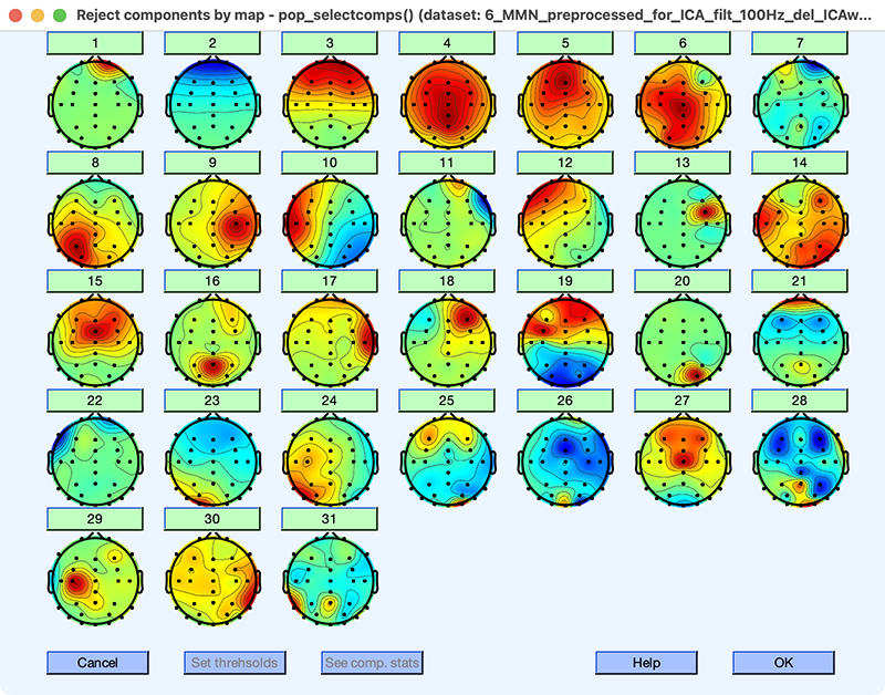
The first thing you should notice is that many of the maps are irregular, even in the top half of the ICs (e.g., ICs 6, 7, and 14). That’s a strong hint that the decomposition did not work well. The next thing you should note is that IC 1 (which must account for a lot of variance, because it’s the first IC) doesn’t have a scalp map that corresponds to a typical artifact or brain signal, with a narrow focus at Fp2. Click on the 1 above the map for IC 1 to see its properties. The time course shows that it is strongly active during a few brief time periods and not at other times. Again, that’s unusual.

Now look at IC 2 (and click on the 2 above the map to see its properties). It has the kind of scalp map we’d expect for blinks, and the time course contains the kind of distributed bursts that we’d expect for blinks. But note that the weights in the scalp map are negative, whereas we saw positive weights at the frontal sites for blink-related ICs in our previous exercises. This is because the polarity of the IC maps is arbitrary, and a given IC may have either positive weights or negative weights. Just for fun, I repeated the decomposition a second time, and I found that IC 2 had positive weights in this repetition of the decomposition. The polarity of the weights in the maps is completely arbitrary, and the polarity of the activation values will also be reversed to come up with the right voltage polarity when we reconstruct the data. So, reversals of map polarity are not a problem.

To see this, scroll through the IC activations using EEGLAB > Plot > Component activations (scroll). You’ll see that IC 2 has negative deflections at the times of blinks, whereas we saw positive deflections for the blink IC in our previous examples (e.g., Screenshot 9.4). If we multiply the negative activation values by the negative weights for the frontal sites, we’ll get a positive voltage. So, it doesn’t matter if we have positive weights along with positive activations or negative weights along with negative activations. In either case, blinks will be reconstructed as a positive voltage at the frontal sites (but a negative voltage at VEOG-lower).

Another thing you should notice in the IC maps is that there isn’t an IC with the scalp topography we’d expect for horizontal eye movements. There were many clear horizontal eye movements in the HEOG-bipolar channel when we scrolled through the data, but we haven’t captured these eye movements as a distinct IC in this decomposition. That also indicates that it didn’t work well. Some participants don’t have many horizontal eye movements, and the lack of an IC for horizontal eye movements would not be a problem for those participants.)

Now let’s try to improve the decomposition by deleting the time periods with the huge C.R.A.P. artifacts. Make 6_MMN_preprocessed_filt_100Hz_del the active dataset and select EEGLAB > ERPLAB > Preprocess EEG > Artifact rejection (continuous EEG). This routine is like the moving window peak-to-peak amplitude routine for artifact detection that we used in the previous chapter, but with two differences. First, it operates on continuous EEG rather than epoched EEG. Second, it eventually deletes sections of the data with artifacts rather than simply marking them.

In the window that appears for this routine, enter 500 as the threshold. We’re not trying to reject blinks or other ordinary artifacts, so we need a much higher threshold for this routine than we would use for normal artifact detection. 500 is a good starting threshold, but you may need to adjust it for some participants. Enter 1000 for the moving window width and 500 as the step size. This will cause it to look for 1000-ms time periods in which the peak-to-peak voltage exceeds the threshold, shifting the window in 500-ms increments. Finally, enter 1:31 for the channels. We’re going to exclude Channels 32 and 33 (the bipolar EOG channels) when we do the ICA decomposition, so we don’t care about huge C.R.A.P. in these channels. (You might also want to exclude Fp1 and Fp2 if you have such large blinks in these channels that blinks end up exceeding the threshold for rejection.) Leave all the check boxes unchecked, and click ACCEPT to run the routine.

When it finishes, you should see in the Matlab command window that the routine has found 15 segments of data to reject. At this point, these segments have just been marked, but they will be deleted when we save the dataset. You should also see a window for scrolling through the marked dataset. If you scroll through the data, you’ll see segments of data that are marked in yellow at ~70 and ~72 seconds (as well as at 96, 254, 403, and 413 seconds). These are the time periods where we saw the huge C.R.A.P., so the artifact rejection routine is working well.

There’s one thing that’s a little odd, though, namely that we’ll delete the data from ~70-71 seconds and from ~71.5-73 seconds, leaving just a 500 ms of unrejected data in the middle. The rejection routine has a feature for avoiding this kind of oddity. Let’s give it a try. First, close the scrolling plot window and cancel the window for saving the dataset. Now select EEGLAB > ERPLAB > Preprocess EEG > Artifact rejection (continuous EEG) again. Keep the parameters the same, but check the box labeled Join artifactual segments separated by less than and put 1000 in the corresponding text box. This will cause any segments of <1000 ms between deleted segments to be deleted. Click ACCEPT to run the routine. Now you should see that a single continuous segment from ~70-73 ms now has been marked for deletion instead of two separate but nearby segments.

To actually delete the marked segments, go to the window that appeared for saving the new dataset and save it with the default name. Now go to EEGLAB > Plot > Channel data (scroll) and look at the result of the artifact rejection you just performed. If you look at the 5-second period starting at 68 seconds, you’ll see that the artifactual activity at ~70 seconds is gone and has been replaced with a boundary event, which has been inserted to mark the discontinuity in the data that was produced by deleting the segment from ~70-73 seconds.

Note that you can also manually reject sections with huge C.R.A.P. using EEGLAB > Tools > Inspect/reject data by eye. ERPLAB’s Artifact rejection (continuous EEG) routine is faster and more easily scriptable than the manual rejection routine, but sometimes it’s useful to do it manually instead (or in addition). Just remember that your goal is to delete segments that will cause problems for ICA, not to delete segments with ordinary artifacts. That is, you want to delete segments with voltage deflections that are large and infrequent, especially if they have an inconsistent scalp distribution.

Now let’s see how deleting the huge C.R.A.P. has impacted the ICA decomposition. You can see the resulting decomposition by loading the dataset named 6_MMN_preprocessed_filt_100Hz_del_car_ICAweights and then selecting using EEGLAB > Tools > Inspect/label components by map. The scalp maps are shown in Screenshot 9.10.

Screenshot 9.10

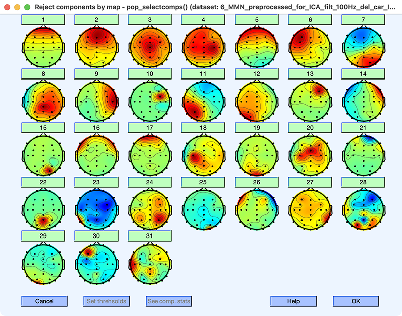
The first thing to notice is that the scalp maps are more regular than those we obtained without deleting the huge C.R.A.P. (see Screenshot 9.9). There are still some irregular maps, but mainly in the bottom half, which don’t account for much variance (e.g., ICs 20 and 23). The second thing to notice is that IC 1 is now a blink component. And the third thing to notice is that we now have an IC with the usual scalp map for horizontal eye movements (IC 14). So, by deleting segments with huge C.R.A.P., we obtained a much better ICA decomposition, even though we only deleted ~10 seconds worth of data.

The next step is to transfer the ICA weights to the original dataset (which are in a file named 6_MMN_preprocessed). Then you should scroll through the data and component activations (simultaneously) to begin the process of determining which ICs to exclude from the reconstructed data.

Go ahead and remove IC 1 (EEGLAB > Tools > Remove components from data), and then scroll through the resulting dataset. Note that this dataset has the break periods at the beginning and end, so the huge C.R.A.P. artifacts are now about 10 seconds later than before.

You should see that the blink correction has done a good job of eliminating the voltages produced by ordinary blinks. However, the periods with huge C.R.A.P. artifacts are still present and still have large artifacts. You would therefore want to perform artifact detection on the epoched data to mark these epochs and then reject them in the averaging process.