Ordinarily, you would decide exactly how to quantify and analyze the ERP amplitudes and latencies prior to seeing the data. If you first look at the grand average ERP waveforms, the analysis parameters you select will likely be influenced by noise in the data, and you’ll have a high likelihood of finding significant effects that reflect noise rather than true effects and are completely bogus. This is a super important point! I’m not going to dwell on it here, because I’ve written about it extensively elsewhere (see especially Luck & Gaspelin, 2017). However, keep this point in mind throughout the chapter (especially in this first exercise, where we are going to look at the data before we develop our analysis plan—exactly what you shouldn’t do!).
I’ve already created the averaged ERP waveforms for looking at the LRP. If you go to the Chapter_10 folder, you’ll see a subfolder named Data, and inside that subfolder you’ll see another subfolder named ERPsets that contains an ERPset for each of the 40 participants. To create these ERPsets, I referenced the data to the average of P9 and P10, high-pass filtered at 0.1 Hz (12 dB/octave), and then applied ICA-based artifact correction for blinks and horizontal eye movements (using the optimized approach described in the chapter on artifact correction). The next step was to add an EventList and then run BINLISTER to create 4 bins:
Bin 1: Left-Pointing Target with Compatible Flankers, Followed by Left Response
Bin 2: Right-Pointing Target with Compatible Flankers, Followed by Right Response
Bin 3: Left-Pointing Target with Incompatible Flankers, Followed by Left Response
Bin 4: Right-Pointing Target with Incompatible Flankers, Followed by Right Response
Note that only correct responses were included in these bins because we’re going to focus on the LRP rather than the ERN.
Next, I epoched the data from -200 to 800 ms relative to stimulus onset. I then performed artifact detection to mark trials with C.R.A.P., and finally I averaged the data, excluding the marked trials.
Let’s load the data and make a grand average. Quit and restart EEGLAB, and set Chapter_10 to be Matlab’s current folder. Select EEGLAB > ERPLAB > Load existing ERPset, navigate to the Chapter_10 > Data > ERPsets folder, select all 40 ERPset files at once, and click Open. You should then be able to see all 40 ERPsets in the ERPsets menu. To make a grand average, select EEGLAB > ERPLAB > Average across ERPsets (Grand Average), and indicate that the routine should average across ERPsets 1:40 in the ERPsets menu. All the other options should be kept at their default values. Click RUN and name the resulting ERPset grand. Save it as a file named grand.erp, because you’ll need it for a later exercise. Now plot the ERPs (EEGLAB > ERPLAB > Plot ERP > Plot ERP waveforms), making one plot for Bins 1 and 2 (compatible trials) and another plot for Bins 3 and 4 (incompatible trials). Find the C3 and C4 channels (where the LRP is typically largest) and look for the contralateral negativity from ~200-400 ms.
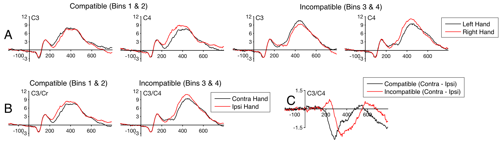
The key waveforms are summarized in Figure 10.2.A. For the compatible trials, the voltage at C3 from ~200-400 ms is more negative on trials with a right-hand response than on trials with a left-hand response, and the voltage at C4 during this period is more negative on trials with a left-hand response than on trials with a right-hand response. The overall voltage is positive in this time range (because of the P3b component), and the LRP sums with the positive voltages to make the voltage more negative (less positive) over the contralateral hemisphere than over the ipsilateral hemisphere.
The pattern is a little more complicated for the incompatible trials. At approximately 200 ms, you can see an opposite-polarity effect, with a more negative voltage for left-hand than for right-hand responses at C3 and a more negative voltage for right-hand than for left-hand responses at C4. This then reverses beginning at approximately 250 ms.
Figure 10.2. Grand averages from the new analysis of the ERP CORE flankers experiment, time-locked to stimulus onset. (A) Original parent waveforms. (B) Waveforms after collapsing into contralateral and ipsilateral hemispheres (relative to response hand). (C) Contralateral-minus-ipsilateral difference waves.
It’s a little challenging to piece together everything that’s happening with the waveforms shown in Figure 10.2.A. There are just a lot of waveforms to look at. We can simplify things by using ERP Bin Operations to collapse the data into contralateral waveforms (left-hemisphere waveforms on right-response trials averaged with right-hemisphere waveforms on left-response trials) and ipsilateral waveforms (left-hemisphere waveforms on left-response trials averaged with right-hemisphere waveforms on right-response trials).
Making these collapsed ERPsets is a little tricky (and is explained in the ERP Bin Operations section of the ERPLAB Manual). To save some of your time, I’ve already made these collapsed ERPsets for you. To open them, first clear out any existing ERPsets from ERPLAB using EEGLAB > ERPLAB > Clear ERPset(s). You should have 41 ERPsets (which you can verify in the ERPsets menu), so enter 1:41 when asked which ERPsets to clear. Next, load the 40 ERPsets in the Chapter_10 > Data > ERPsets_CI folder. You can now make a grand average of these ERPsets and plot the results (with one plot for Bins 1 and 2, and a separate plot for Bins 3 and 4).
Figure 10.2.B shows the results from the C3 and C4 electrode sites (which are now combined, as indicated by the C3/C4 label). Now we have only two pairs of waveforms rather than four pairs of waveforms, which makes it easier to see the contralateral negativity.
To make things even easier, and to isolate the LRP from other overlapping voltages, we can use ERP Bin Operations make a contralateral-minus-ipsilateral difference wave (Bin 1 minus Bin 2 for the compatible trials, and Bin 3 minus Bin 4 for the ipsilateral trials). I’ve already done this for you. Clear out the ERPsets and load these difference wave files from the Chapter_10 > Data > ERPsets_CI_Diff folder. Make a grand average, and plot the results (in a single plot with Bins 1 and 2).
Figure 10.2.C. shows the results at C3/C4. Now we have only one pair of waveforms, making it much easier to compare the LRP for the compatible and incompatible trials. On the compatible trials, you can see a nice clear negativity from ~200-500 ms. On the incompatible trials, you can see an initial contralateral positivity (which is really a negativity relative to the incorrect response), followed by a delayed contralateral negativity.
This is pretty cool! Our main goal in including both compatible and incompatible trials in this experiment was to generate a sufficient number of errors for the ERN analysis (because errors are a lot more common on incompatible trials). We didn’t intend to do any comparisons of compatible and incompatible trials, so this is the first time anyone has looked at these effects. It’s gratifying to see that we found the same pattern as in prior studies (e.g., Gratton et al., 1988), with a delayed LRP on incompatible trials that is preceded by an opposite-polarity deflection.