2.3: From the Laws of Thought to Binary Logic

In 1854, with the publication of An Investigation of the Laws of Thought, George Boole (2003) invented modern mathematical logic. Boole’s goal was to move the study of thought from the domain of philosophy into the domain of mathematics:

There is not only a close analogy between the operations of the mind in general reasoning and its operations in the particular science of Algebra, but there is to a considerable extent an exact agreement in the laws by which the two classes of operations are conducted. (Boole, 2003, p. 6)

Today we associate Boole’s name with the logic underlying digital computers (Mendelson, 1970). However, Boole’s algebra bears little resemblance to our modern interpretation of it. The purpose of this section is to trace the trajectory that takes us from Boole’s nineteenth-century calculus to the twentieth-century invention of truth tables that define logical functions over two binary inputs.

Boole did not create a binary logic; instead he developed an algebra of sets. Boole used symbols such as \(x,\,y,\) and \(z\) to represent classes of entities. He then defined “signs of operation, as +, –, ´, standing for those operations of the mind by which the conceptions of things are combined or resolved so as to form new conceptions involving the same elements” (Boole, 2003, p. 27). The operations of his algebra were those of election: they selected subsets of entities from various classes of interest (Lewis, 1918).

For example, consider two classes: \(x\) (e.g., “black things”) and \(y\) (e.g., “birds”). Boole’s expression \(x\,+\,y\) performs an “exclusive or” of the two constituent classes, electing the entities that were “black things,” or were “birds,” but not those that were “black birds.”

Elements of Boole’s algebra pointed in the direction of our more modern binary logic. For instance, Boole used multiplication to elect entities that shared properties defined by separate classes. So, continuing our example, the set of “black birds” would be elected by the expression \(xy\). Boole also recognized that if one multiplied a class with itself, the result would simply be the original set again. Boole wrote his fundamental law of thought as \(xx\,=\,x\), which can also be expressed as \(x^2\,=\,x\). He realized that if one assigned numerical quantities to \(x\), then this law would only be true for the values 0 and 1. “Thus it is a consequence of the fact that the fundamental equation of thought is of the second degree, that we perform the operation of analysis and classification, by division into pairs of opposites, or, as it is technically said, by dichotomy” (Boole, 2003, pp. 50–51). Still, this dichotomy was not to be exclusively interpreted in terms of truth or falsehood, though Boole exploited this representation in his treatment of secondary propositions. Boole typically used 0 to represent the empty set and 1 to represent the universal set; the expression \(1\,–\,x\) elected those entities that did not belong to \(x\).

Boole’s operations on symbols were purely formal. That is, the actions of his logical rules were independent of any semantic interpretation of the logical terms being manipulated.

We may in fact lay aside the logical interpretation of the symbols in the given equation; convert them into quantitative symbols, susceptible only of the values 0 and 1; perform upon them as such all the requisite processes of solution; and finally restore to them their logical interpretation. (Boole, 2003, p. 70)

This formal approach is evident in Boole’s analysis of his fundamental law. Beginning with \(x^2\,=\,x\), Boole applied basic algebra to convert this expression into \(x\,–\,x^2\,=\,0\). He then simplified this expression to \(x(1\,–\,x)\,=\,0\). Note that none of these steps are logical in nature; Boole would not be able to provide a logical justification for his derivation. However, he did triumphantly provide a logical interpretation of his result: 0 is the empty set, 1 the universal set, \(x\) is some set of interest, and \(1\,–\,x\) is the negation of this set. Boole’s algebraic derivation thus shows that the intersection of \(x\) with its negation is the empty set. Boole noted that, in terms of logic, the equation \(x(1\,–\,x)\,=\,0\) expressed,

that it is impossible for a being to possess a quality and not to possess that quality at the same time. But this is identically that ‘principle of contradiction’ which Aristotle has described as the fundamental axiom of all philosophy. (Boole, 2003, p. 49)

It was important for Boole to link his calculus to Aristotle, because Boole not only held Aristotelian logic in high regard, but also hoped that his new mathematical methods would both support Aristotle’s key logical achievements as well as extend Aristotle’s work in new directions. To further link his formalism to Aristotle’s logic, Boole applied his methods to what he called secondary propositions. A secondary proposition was a statement about a proposition that could be either true or false. As a result, Boole’s analysis of secondary propositions provides another glimpse of how his work is related to our modern binary interpretation of it.

Boole applied his algebra of sets to secondary propositions by adopting a temporal interpretation of election. That is, Boole considered that a secondary proposition could be true or false for some duration of interest. The expression \(xy\) would now be interpreted as electing a temporal period during which both propositions \(x\) and \(y\) are true. The symbols 0 and 1 were also given temporal interpretations, meaning “no time” and “the whole of time” respectively. While this usage differs substantially from our modern approach, it has been viewed as the inspiration for modern binary logic (Post, 1921).

Boole’s work inspired subsequent work on logic in two different ways. First, Boole demonstrated that an algebra of symbols was possible, productive, and worthy of exploration: “Boole showed incontestably that it was possible, by the aid of a system of mathematical signs, to deduce the conclusions of all these ancient modes of reasoning, and an indefinite number of other conclusions” (Jevons, 1870, p. 499). Second, logicians noted certain idiosyncrasies of and deficiencies with Boole’s calculus, and worked on dealing with these problems. Jevons also wrote that Boole’s examples “can be followed only by highly accomplished mathematical minds; and even a mathematician would fail to find any demonstrative force in a calculus which fearlessly employs unmeaning and incomprehensible symbols” (p. 499). Attempts to simplify and correct Boole produced new logical systems that serve as the bridge between Boole’s nineteenth-century logic and the binary logic that arose in the twentieth century.

Boole’s logic is problematic because certain mathematical operations do not make sense within it (Jevons, 1870). For instance, because addition defined the “exclusive or” of two sets, the expression \(x\,+\,x\) had no interpretation in Boole’s system. Jevons believed that Boole’s interpretation of addition was deeply mistaken and corrected this by defining addition as the “inclusive or” of two sets. This produced an interpretable additive law, \(x\,+\,x\,=\,x\), that paralleled Boole’s multiplicative fundamental law of thought.

Jevons’ (1870) revision of Boole’s algebra led to a system that was simple enough to permit logical inference to be mechanized. Jevons illustrated this with a three-class system, in which upper-case letters (e.g., \(A\)) picked out those entities that belonged to a set and lower-case letters (e.g., \(a\)) picked out those entities that did not belong. He then produced what he called the logical abecedarium, which was the set of possible combinations of the three classes. In his three-class example, the abecedarium consisted of eight combinations: \(ABC,\,ABc,\,AbC,\,Abc,\,aBC,\,aBc,\,abC,\) and \(abc\). Note that each of these combinations is a multiplication of three terms in Boole’s sense, and thus elects an intersection of three different classes. As well, with the improved definition of logical addition, different terms of the abecedarium could be added together to define some set of interest. For example Jevons (but not Boole!) could elect the class \(B\) with the following expression: \(B\,=\,ABC\,+\,ABc\,+\,aBC\,+\,aBc\).

Jevons (1870) demonstrated how the abecedarium could be used as an inference engine. First, he used his set notation to define concepts of interest, such as in the example \(A\) = iron, \(B\) = metal, and \(C\) = element. Second, he translated propositions into intersections of sets. For instance, the premise “Iron is metal” can be rewritten as “\(A\) is \(B\),” which in Boole’s algebra becomes \(AB\), and “metal is element” becomes \(BC\). Third, given a set of premises, Jevons removed the terms that were inconsistent with the premises from the abecedarium: the only terms consistent with the premises \(AB\) and \(BC\) are \(ABC,\,aBC,\,abC,\)and \(abc\). Fourth, Jevons inspected and interpreted the remaining abecedarium terms to perform valid logical inferences. For instance, from the four remaining terms in Jevons’ example, we can conclude that “all iron is element,” because \(A\) is only paired with \(C\) in the terms that remain, and “there are some elements that are neither metal nor iron,” or \(abC\). Of course, the complete set of entities that is elected by the premises is the logical sum of the terms that were not eliminated.

Jevons (1870) created a mechanical device to automate the procedure described above. The machine, known as the “logical piano” because of its appearance, displayed the 16 different combinations of the abecedarium for working with four different classes. Premises were entered by pressing keys; the depression of a pattern of keys removed inconsistent abecedarium terms from view. After all premises had been entered in sequence, the terms that remained on display were interpreted. A simpler variation of Jevons’ device, originally developed for four-class problems but more easily extendable to larger situations, was invented by Allan Marquand (Marquand, 1885). Marquand later produced plans for an electric version of his device that used electromagnets to control the display (Mays, 1953). Had this device been constructed, and had Marquand’s work come to the attention of a wider audience, the digital computer might have been a nineteenth-century invention (Buck & Hunka, 1999).

With respect to our interest in the transition from Boole’s work to our modern interpretation of it, note that the logical systems developed by Jevons, Marquand, and others were binary in two different senses. First, a set and its complement (e.g., \(A\) and \(a\)) never co-occurred in the same abecedarium term. Second, when premises were applied, an abecedarium term was either eliminated or not. These binary characteristics of such systems permitted them to be simple enough to be mechanized.

The next step towards modern binary logic was to adopt the practice of assuming that propositions could either be true or false, and to algebraically indicate these states with the values 1 and 0. We have seen that Boole started this approach, but that he did so by applying awkward temporal set-theoretic interpretations to these two symbols.

The modern use of 1 and 0 to represent true and false arises later in the nineteenth century. British logician Hugh McColl’s (1880) symbolic logic used this notation, which he borrowed from the mathematics of probability. American logician Charles Sanders Peirce (1885) also explicitly used a binary notation for truth in his famous paper “On the algebra of logic: A contribution to the philosophy of notation.” This paper is often cited as the one that introduced the modern usage (Ewald, 1996). Peirce extended Boole’s work on secondary propositions by stipulating an additional algebraic law of propositions: for every element \(x\), either \(x\,=\,0\) or \(x\,=\,1\), producing a system known as “the two-valued algebra” (Lewis, 1918).

The two-valued algebra led to the invention of truth tables, which are established in the literature in the early 1920s (Post, 1921; Wittgenstein, 1922), but were likely in use much earlier. There is evidence that Bertrand Russell and his then student Ludwig Wittgenstein were using truth tables as early as 1910 (Shosky, 1997). It has also been argued that Charles Peirce and his students probably were using truth tables as early as 1902 (Anellis, 2004).

Truth tables make explicit an approach in which primitive propositions (\(p,\,q,\,r,\) etc.) that could only adopt values of 0 or 1 are used to produce more complex expressions. These expressions are produced by using logical functions to combine simpler terms. This approach is known as “using truth-value systems” (Lewis & Langford, 1959). Truth-value systems essentially use truth tables to determine the truth of functions of propositions (i.e., of logical combinations of propositions). “It is a distinctive feature of this two-valued system that when the property, 0 or 1, of the elements \(p,\,q,\) etc., is given, any function of the elements which is in the system is thereby determined to have the property 0 or the property 1” (p. 199).

Consider Table \(PageIndex{1}\), which provides the values of three different functions (the last three columns of the table) depending upon the truth value of two simple propositions (the first two columns of the table):

\(p\)	\(q\)	\(p\cdot q\)	\(p+q\)	\(p\cdot (p+q)\)
1	1	1	1	1
1	0	0	1	1
0	1	0	1	0
0	0	0	0	0

Table 1. Examples of the truth value system for two elementary propositions and some of their combinations. The possible values of p and q are given in the first two columns. The resulting values of different functions of these propositions are provided in the remaining columns.

Truth-value systems result in a surprising, simplified approach to defining basic or primitive logical functions. When the propositions p and q are interpreted as being only true or false, then there are only four possible combinations of these two propositions that can exist, i.e., the first two columns of Table \(PageIndex{1}\). A primitive function can be defined as a function that is defined over p and q, and that takes on a truth value for each combination of these variables.

Given that in a truth-value system a function can only take on the value of 0 or 1, then there are only 16 different primitive functions that can be defined for combinations of the binary inputs p and q (Ladd, 1883). These primitive functions are provided in Table \(PageIndex{2}\); each row of the table shows the truth values of each function for each combination of the inputs. An example logical notation for each function is provided in the last column of the table. This notation was used by Warren McCulloch (1988b), who attributed it to earlier work by Wittgenstein.

Not surprisingly, an historical trajectory can also be traced for the binary logic defined in Table \(PageIndex{2}\). Peirce’s student Christine Ladd actually produced the first five columns of that table in her 1883 paper, including the conversion of the first four numbers in a row from a binary to a base 10 number. However, Ladd did not interpret each row as defining a logical function. Instead, she viewed the columns in terms of set notation and each row as defining a different “universe.” The interpretation of the first four columns as the truth values of various logical functions arose later with the popularization of truth tables (Post, 1921; Wittgenstein, 1922).

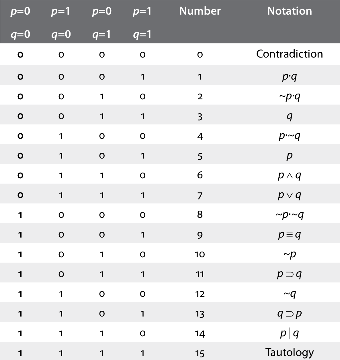
Table 2. Truth tables for all possible functions of pairs of propositions. Each function has a truth value for each possible combination of the truth values of p and q, given in the first four columns of the table. The Number column converts the first four values in a row into a binary number (Ladd, 1883). The logical notation for each function is taken Warren McCulloch (1988b).

Truth tables, and the truth-value system that they support, are very powerful. They can be used to determine whether any complex expression, based on combinations of primitive propositions and primitive logical operations, is true or false (Lewis, 1932). In the next section we see the power of the simple binary truth-value system, because it is the basis of the modern digital computer. We also see that bringing this system to life in a digital computer leads to the conclusion that one must use more than one vocabulary to explain logical devices.