4.8: What Do Output Unit Activities Represent?

When McCulloch and Pitts (1943) formalized the information processing of neurons, they did so by exploiting the all-or-none law. As a result, whether a neuron responded could be interpreted as assigning a “true” or “false” value to some proposition computed over the neuron’s outputs. McCulloch and Pitts were able to design artificial neurons capable of acting as 14 of the 16 possible primitive functions on the two-valued logic that was described in Chapter 2.

McCulloch and Pitts (1943) formalized the all-or-none law by using the Heaviside step equation as the activation function for their artificial neurons. Modern activation functions such as the logistic equation provide a continuous approximation of the step function. It is also quite common to interpret the logistic function in digital, step function terms. This is done by interpreting a modern unit as being “on” or “off ” if its activity is sufficiently extreme. For instance, in simulations conducted with my laboratory software (Dawson, 2005) it is typical to view a unit as being “on” if its activity is 0.9 or higher, or “off ” if its activity is 0.1 or lower.

Digital activation functions, or digital interpretations of continuous activation functions, mean that pattern recognition is a primary task for artificial neural networks (Pao, 1989; Ripley, 1996). When a network performs pattern recognition, it is trained to generate a digital or binary response to an input pattern, where this response is interpreted as representing a class to which the input pattern is unambiguously assigned.

What does the activity of a unit in a connectionist network mean? Under the strict digital interpretation described above, activity is interpreted as the truth value of some proposition represented by the unit. However, modern activation functions such as the logistic or Gaussian equations have continuous values, which permit more flexible kinds of interpretation. Continuous activity might model the frequency with which a real unit (i.e., a neuron) generates action potentials. It could represent a degree of confidence in asserting that a detected feature is present, or it could represent the amount of a feature that is present (Waskan & Bechtel, 1997).

In this section, a computational-level analysis is used to prove that, in the context of modern learning theory, continuous unit activity can be unambiguously interpreted as a candidate measure of degree of confidence with conditional probability (Waskan & Bechtel, 1997).

In experimental psychology, some learning theories are motivated by the ambiguous or noisy nature of the world. Cues in the real world do not signal outcomes with complete certainty (Dewey, 1929). It has been argued that adaptive systems deal with worldly uncertainty by becoming “intuitive statisticians,” whether these systems are humans (Peterson & Beach, 1967) or animals (Gallistel, 1990; Shanks, 1995). An agent that behaves like an intuitive statistician detects contingency in the world, because cues signal the likelihood (and not the certainty) that certain events (such as being rewarded) will occur (Rescorla, 1967, 1968).

Evidence indicates that a variety of organisms are intuitive statisticians. For example, the matching law is a mathematical formalism that was originally used to explain variations in response frequency. It states that the rate of a response reflects the rate of its obtained reinforcement. For instance, if response A is reinforced twice as frequently as response B, then A will appear twice as frequently as B (Herrnstein, 1961). The matching law also predicts how response strength varies with reinforcement frequency (de Villiers & Herrnstein, 1976). Many results show that the matching law governs numerous tasks in psychology and economics (Davison & McCarthy, 1988; de Villiers, 1977; Herrnstein, 1997).

Another phenomenon that is formally related (Herrnstein & Loveland, 1975) to the matching law is probability matching, which concerns choices made by agents faced with competing alternatives. Under probability matching, the likelihood that an agent makes a choice amongst different alternatives mirrors the probability associated with the outcome or reward of that choice (Vulkan, 2000). Probability matching has been demonstrated in a variety of organisms, including insects (Fischer, Couvillon,&Bitterman, 1993; Keasar et al., 2002; Longo, 1964; Niv et al., 2002), fish (Behrend & Bitterman, 1961), turtles (Kirk&Bitterman, 1965), pigeons (Graf, Bullock, & Bitterman, 1964), and humans (Estes&Straughan, 1954).

Perceptrons, too, can match probabilities (Dawson et al., 2009). Dawson et al. used four different cues, or discriminative stimuli (DSs), but did not “reward” them 100 percent of the time. Instead, they rewarded one DS 20 percent of the time, another 40 percent, a third 60 percent, and a fourth 80 percent. After 300 epochs, where each epoch involved presenting each cue alone 10 different times in random order, these contingencies were inverted (i.e., subtracted from 100). The dependent measure was perceptron activity when a cue was presented; the activation function employed was the logistic. Some results of this experiment are presented in Figure 4-6. It shows that after a small number of epochs, the output unit activity becomes equal to the probability that a presented cue was rewarded. It also shows that perceptron responses quickly readjust when contingencies are suddenly modified, as shown by the change in Figure 4-6 around epoch 300. In short, perceptrons are capable of probability matching.

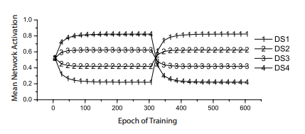
Figure 4-6. Probability matching by perceptrons. Each line shows the perceptron activation when a different cue (or discriminative stimulus, DS) is presented. Activity levels quickly become equal to the probability that each cue was reinforced (Dawson et al., 2009).

That perceptrons match probabilities relates them to contingency theory. Formal statements of this theory formalize contingency as a contrast between conditional probabilities (Allan, 1980; Cheng, 1997; Cheng & Holyoak, 1995; Cheng & Novick, 1990, 1992; Rescorla, 1967, 1968).

For instance, consider the simple situation in which a cue can either be presented, C, or not, ~C. Associated with either of these states is an outcome (e.g., a reward) that can either occur, O, or not, ~O. In this simple situation, involving a single cue and a single outcome, the contingency between the cue and the outcome is formally defined as the difference in conditional probabilities, ΔP, where ΔP = P(O|C) – P(O|~C) (Allan, 1980). More sophisticated models, such as the probabilistic contrast model (e.g., Cheng & Novick, 1990) or the power PC theory (Cheng, 1997), Epoch of Training Mean Network Activation define more complex probabilistic contrasts that are possible when multiple cues occur and can be affected by the context in which they are presented.

Empirically, the probability matching of perceptrons, illustrated in Figure 4-6, suggests that their behaviour can represent ΔP. When a cue is presented, activity is equal to the probability that the cue signals reinforcement—that is, P(O|C). This implies that the difference between a perceptron’s activity when a cue is presented and its activity when a cue is absent must be equal to ΔP. Let us now turn to a computational analysis to prove this claim.

What is the formal relationship between formal contingency theories and theories of associative learning (Shanks, 2007)? Researchers have compared the predictions of an influential account of associative learning, the Rescorla-Wagner model (Rescorla & Wagner, 1972), to formal theories of contingency (Chapman & Robbins, 1990; Cheng, 1997; Cheng & Holyoak, 1995). It has been shown that while in some instances the Rescorla-Wagner model predicts the conditional contrasts defined by a formal contingency theory, in other situations it fails to generate these predictions (Cheng, 1997).

Comparisons between contingency learning and Rescorla-Wagner learning typically involve determining equilibria of the Rescorla-Wagner model. An equilibrium of the Rescorla-Wagner model is a set of associative strengths defined by the model, at the point where the asymptote of changes in error defined by RescorlaWagner learning approaches zero (Danks, 2003). In the simple case described earlier, involving a single cue and a single outcome, the Rescorla-Wagner model is identical to contingency theory. This is because at equilibrium, the associative strength between cue and outcome is exactly equal to ΔP (Chapman & Robbins, 1990).

There is also an established formal relationship between the Rescorla-Wagner model and the delta rule learning of a perceptron (Dawson, 2008; Gluck & Bower, 1988; Sutton & Barto, 1981). Thus by examining the equilibrium state of a perceptron facing a simple contingency problem, we can formally relate this kind of network to contingency theory and arrive at a formal understanding of what output unit activity represents.

When a continuous activation function is used in a perceptron, calculus can be used to determine the equilibrium of the perceptron. Let us do so for a single cue situation in which some cue, C, when presented, is rewarded a frequency of a times, and is not rewarded a frequency of b times. Similarly, when the cue is not presented, the perceptron is rewarded a frequency of c times and is not rewarded a frequency of d times. Note that to reward a perceptron is to train it to generate a desired response of 1, and that to not reward a perceptron is to train it to generate a desired response of 0, because the desired response indicates the presence or absence of the unconditioned stimulus (Dawson, 2008).

Assume that when the cue is present, the logistic activation function computes an activation value that we designate as oc , and that when the cue is absent it returns the activation value designated as o~c. We can now define the total error of responding for the perceptron, that is, its total error for the (a + b + c + d) number of patterns that represent a single epoch, in which each instance of the contingency problem is presented once. For instance, on a trial in which C is presented and the perceptron is reinforced, the perceptron’s error for that trial is the squared difference between the reward, 1, and o_c. As there are a of these trials, the total contribution of this type of trial to overall error is a(1 – o_c )² . Applying this logic to the other three pairings of cue and outcome, total error E can be defined as follows:

E = a(1-o_c)² + b(0-o_c)² + c(1-o_~c)² + d(0-o_~c)²

= a(1-o_c)² + b(o_c)² + c(1-o_~c)² + d(o_~c)²

For a perceptron to be at equilibrium, it must have reached a state in which total error has been optimized, so that the error can no longer be decreased by using the delta rule to alter the perceptron’s weight. To determine the equilibrium of the perceptron for the single cue contingency problem, we begin by taking the derivative of the error equation with respect to the activity of the perceptron when the cue is present, o_c :

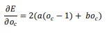
One condition of the perceptron at equilibrium is that oc is a value that causes this derivative to be equal to 0. The equation below sets the derivative to 0 and solves for oc . The result is a/(a + b), which is equal to the conditional probability P(O|C) if the single cue experiment is represented with a traditional contingency table:

Similarly, we can take the derivative of the error equation with respect to the activity of the perceptron when the cue is not present, o~c: ( ) ( ) ( ) ( ) ( ) ( ) ( ) ( ) ) ) ( | ) ( ( ) ) ( ) ( ) ) ) Elements of Connectionist Cognitive Science 157 A second condition of the perceptron at equilibrium is that o~c is a value that causes the derivative above to be equal to 0. As before, we can set the derivative to 0 and solve for the value of o~c. This time the result is c/(c + d), which in a traditional contingency table is equal to the conditional probability P(O|~C): The main implication of the above equations is that they show that perceptron activity is literally a conditional probability. This provides a computational proof for the empirical hypothesis about perceptron activity that was generated from examining Figure 4-6. A second implication of the proof is that when faced with the same contingency problem, a perceptron’s equilibrium is not the same as that for the Rescorla-Wagner model. At equilibrium, the associative strength for the cue C that is determined by Rescorla-Wagner training is literally ΔP (Chapman & Robbins, 1990). This is not the case for the perceptron. For the perceptron, ΔP must be computed by taking the difference between its output when the cue is present and its output when the cue is absent. That is, ΔP is not directly represented as a connection weight, but instead is the difference between perceptron behaviours under different cue situations— that is, the difference between the conditional probability output by the perceptron when a cue is present and the conditional probability output by the perceptron when the cue is absent. Importantly, even though the perceptron and the Rescorla-Wagner model achieve different equilibria for the same problem, it is clear that both are sensitive to contingency when it is formally defined as ΔP. Differences between the two reflect an issue that was raised in Chapter 2, that there exist many different possible algorithms for computing the same function. Key differences between the perceptron and the Rescorla-Wagner model—in particular, the fact that the former performs a nonlinear transformation on internal signals, while the latter does not—cause them to adopt very different structures, as indicated by different equilibria. Nonetheless, these very different systems are equally sensitive to exactly the same contingency. This last observation has implications for the debate between contingency theory and associative learning (Cheng, 1997; Cheng & Holyoak, 1995; Shanks, 2007). In ( ( ) ) ( ) ( ) ( | ) 158 Chapter 4 the current phase of this debate, modern contingency theories have been proposed as alternatives to Rescorla-Wagner learning. While in some instances equilibria for the Rescorla-Wagner model predict the conditional contrasts defined by a formal contingency theory like the power PC model, in other situations this is not the case (Cheng, 1997). However, the result above indicates that differences in equilibria do not necessarily reflect differences in system abilities. Clearly equilibrium differences cannot be used as the sole measure when different theories of contingency are compared.