12.19: Reading- Illustrating Monopoly Profits
- Page ID
- 162499
\( \newcommand{\vecs}[1]{\overset { \scriptstyle \rightharpoonup} {\mathbf{#1}} } \)
\( \newcommand{\vecd}[1]{\overset{-\!-\!\rightharpoonup}{\vphantom{a}\smash {#1}}} \)
\( \newcommand{\dsum}{\displaystyle\sum\limits} \)
\( \newcommand{\dint}{\displaystyle\int\limits} \)
\( \newcommand{\dlim}{\displaystyle\lim\limits} \)
\( \newcommand{\id}{\mathrm{id}}\) \( \newcommand{\Span}{\mathrm{span}}\)
( \newcommand{\kernel}{\mathrm{null}\,}\) \( \newcommand{\range}{\mathrm{range}\,}\)
\( \newcommand{\RealPart}{\mathrm{Re}}\) \( \newcommand{\ImaginaryPart}{\mathrm{Im}}\)
\( \newcommand{\Argument}{\mathrm{Arg}}\) \( \newcommand{\norm}[1]{\| #1 \|}\)
\( \newcommand{\inner}[2]{\langle #1, #2 \rangle}\)
\( \newcommand{\Span}{\mathrm{span}}\)
\( \newcommand{\id}{\mathrm{id}}\)
\( \newcommand{\Span}{\mathrm{span}}\)
\( \newcommand{\kernel}{\mathrm{null}\,}\)
\( \newcommand{\range}{\mathrm{range}\,}\)
\( \newcommand{\RealPart}{\mathrm{Re}}\)
\( \newcommand{\ImaginaryPart}{\mathrm{Im}}\)
\( \newcommand{\Argument}{\mathrm{Arg}}\)
\( \newcommand{\norm}[1]{\| #1 \|}\)
\( \newcommand{\inner}[2]{\langle #1, #2 \rangle}\)
\( \newcommand{\Span}{\mathrm{span}}\) \( \newcommand{\AA}{\unicode[.8,0]{x212B}}\)
\( \newcommand{\vectorA}[1]{\vec{#1}} % arrow\)
\( \newcommand{\vectorAt}[1]{\vec{\text{#1}}} % arrow\)
\( \newcommand{\vectorB}[1]{\overset { \scriptstyle \rightharpoonup} {\mathbf{#1}} } \)
\( \newcommand{\vectorC}[1]{\textbf{#1}} \)
\( \newcommand{\vectorD}[1]{\overrightarrow{#1}} \)
\( \newcommand{\vectorDt}[1]{\overrightarrow{\text{#1}}} \)
\( \newcommand{\vectE}[1]{\overset{-\!-\!\rightharpoonup}{\vphantom{a}\smash{\mathbf {#1}}}} \)
\( \newcommand{\vecs}[1]{\overset { \scriptstyle \rightharpoonup} {\mathbf{#1}} } \)
\(\newcommand{\longvect}{\overrightarrow}\)
\( \newcommand{\vecd}[1]{\overset{-\!-\!\rightharpoonup}{\vphantom{a}\smash {#1}}} \)
\(\newcommand{\avec}{\mathbf a}\) \(\newcommand{\bvec}{\mathbf b}\) \(\newcommand{\cvec}{\mathbf c}\) \(\newcommand{\dvec}{\mathbf d}\) \(\newcommand{\dtil}{\widetilde{\mathbf d}}\) \(\newcommand{\evec}{\mathbf e}\) \(\newcommand{\fvec}{\mathbf f}\) \(\newcommand{\nvec}{\mathbf n}\) \(\newcommand{\pvec}{\mathbf p}\) \(\newcommand{\qvec}{\mathbf q}\) \(\newcommand{\svec}{\mathbf s}\) \(\newcommand{\tvec}{\mathbf t}\) \(\newcommand{\uvec}{\mathbf u}\) \(\newcommand{\vvec}{\mathbf v}\) \(\newcommand{\wvec}{\mathbf w}\) \(\newcommand{\xvec}{\mathbf x}\) \(\newcommand{\yvec}{\mathbf y}\) \(\newcommand{\zvec}{\mathbf z}\) \(\newcommand{\rvec}{\mathbf r}\) \(\newcommand{\mvec}{\mathbf m}\) \(\newcommand{\zerovec}{\mathbf 0}\) \(\newcommand{\onevec}{\mathbf 1}\) \(\newcommand{\real}{\mathbb R}\) \(\newcommand{\twovec}[2]{\left[\begin{array}{r}#1 \\ #2 \end{array}\right]}\) \(\newcommand{\ctwovec}[2]{\left[\begin{array}{c}#1 \\ #2 \end{array}\right]}\) \(\newcommand{\threevec}[3]{\left[\begin{array}{r}#1 \\ #2 \\ #3 \end{array}\right]}\) \(\newcommand{\cthreevec}[3]{\left[\begin{array}{c}#1 \\ #2 \\ #3 \end{array}\right]}\) \(\newcommand{\fourvec}[4]{\left[\begin{array}{r}#1 \\ #2 \\ #3 \\ #4 \end{array}\right]}\) \(\newcommand{\cfourvec}[4]{\left[\begin{array}{c}#1 \\ #2 \\ #3 \\ #4 \end{array}\right]}\) \(\newcommand{\fivevec}[5]{\left[\begin{array}{r}#1 \\ #2 \\ #3 \\ #4 \\ #5 \\ \end{array}\right]}\) \(\newcommand{\cfivevec}[5]{\left[\begin{array}{c}#1 \\ #2 \\ #3 \\ #4 \\ #5 \\ \end{array}\right]}\) \(\newcommand{\mattwo}[4]{\left[\begin{array}{rr}#1 \amp #2 \\ #3 \amp #4 \\ \end{array}\right]}\) \(\newcommand{\laspan}[1]{\text{Span}\{#1\}}\) \(\newcommand{\bcal}{\cal B}\) \(\newcommand{\ccal}{\cal C}\) \(\newcommand{\scal}{\cal S}\) \(\newcommand{\wcal}{\cal W}\) \(\newcommand{\ecal}{\cal E}\) \(\newcommand{\coords}[2]{\left\{#1\right\}_{#2}}\) \(\newcommand{\gray}[1]{\color{gray}{#1}}\) \(\newcommand{\lgray}[1]{\color{lightgray}{#1}}\) \(\newcommand{\rank}{\operatorname{rank}}\) \(\newcommand{\row}{\text{Row}}\) \(\newcommand{\col}{\text{Col}}\) \(\renewcommand{\row}{\text{Row}}\) \(\newcommand{\nul}{\text{Nul}}\) \(\newcommand{\var}{\text{Var}}\) \(\newcommand{\corr}{\text{corr}}\) \(\newcommand{\len}[1]{\left|#1\right|}\) \(\newcommand{\bbar}{\overline{\bvec}}\) \(\newcommand{\bhat}{\widehat{\bvec}}\) \(\newcommand{\bperp}{\bvec^\perp}\) \(\newcommand{\xhat}{\widehat{\xvec}}\) \(\newcommand{\vhat}{\widehat{\vvec}}\) \(\newcommand{\uhat}{\widehat{\uvec}}\) \(\newcommand{\what}{\widehat{\wvec}}\) \(\newcommand{\Sighat}{\widehat{\Sigma}}\) \(\newcommand{\lt}{<}\) \(\newcommand{\gt}{>}\) \(\newcommand{\amp}{&}\) \(\definecolor{fillinmathshade}{gray}{0.9}\)Illustrating Monopoly Profits
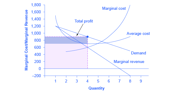
It is straightforward to calculate profits of given numbers for total revenue and total cost. However, the size of monopoly profits can also be illustrated graphically with Figure 9.6, which takes the marginal cost and marginal revenue curves from the previous exhibit and adds an average cost curve and the monopolist’s perceived demand curve.

The three-step process where a monopolist selects the profit-maximizing quantity to produce, decides what price to charge, and then determines total revenue, total cost and profit. These steps include:
Step 1: The Monopolist Determines Its Profit-Maximizing Level of Output
The firm can use the points on the demand curve D to calculate total revenue, and then, based on total revenue, calculate its marginal revenue curve. The profit-maximizing quantity will occur where MR = MC—or at the last possible point before marginal costs start exceeding marginal revenue. On Figure 9.6, MR = MC occurs at an output of 4.
Step 2: The Monopolist Decides What Price to Charge
The monopolist will charge what the market is willing to pay. A dotted line drawn straight up from the profit-maximizing quantity to the demand curve shows the profit-maximizing price. This price is above the average cost curve, which shows that the firm is earning profits.
Step 3: Calculate Total Revenue, Total Cost, and Profit
Total revenue is the overall shaded box, where the width of the box is the quantity being sold and the height is the price. In Figure 9.6, the bottom part of the shaded box, which is shaded more lightly, shows total costs; that is, quantity on the horizontal axis multiplied by average cost on the vertical axis. The larger box of total revenues minus the smaller box of total costs will equal profits, which is shown by the darkly shaded box.
This three-step process is illustrated in Figure 9.7.

In a perfectly competitive market, the forces of entry would erode this profit in the long run. But a monopolist is protected by barriers to entry. In fact, one telltale sign of a possible monopoly is when a firm earns profits year after year, while doing more or less the same thing, without ever seeing those profits eroded by increased competition.
Why is a monopolist’s marginal revenue always less than the price?
The marginal revenue curve for a monopolist always lies beneath the market demand curve. To understand why, think about increasing the quantity along the demand curve by one unit, so that you take one step down the demand curve to a slightly higher quantity but a slightly lower price. A demand curve is not sequential: It is not that first we sell Q1 at a higher price, and then we sell Q2 at a lower price. Rather, a demand curve is conditional: If we charge the higher price, we would sell Q1. If, instead, we charge a lower price (on all the units that we sell), we would sell Q2.
So when we think about increasing the quantity sold by one unit, marginal revenue is affected in two ways. First, we sell one additional unit at the new market price. Second, all the previous units, which could have been sold at the higher price, now sell for less. Because of the lower price on all units sold, the marginal revenue of selling a unit is less than the price of that unit—and the marginal revenue curve is below the demand curve.
Tip: For a straight-line demand curve, the marginal revenue curve equals price at the lowest level of output. (Graphically, MR and demand have the same vertical axis.) As output increases, marginal revenue decreases twice as fast as demand, so that the horizontal intercept of MR is halfway to the horizontal intercept of demand. You can see this in the Figure 9.8.

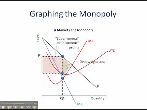
Watch the video below to see these monopoly profits illustrated on a graph.
Self Check: Revenue, Costs, Profit and Losses in Monopolies
Answer the question(s) below to see how well you understand the topics covered in the previous section. This short quiz does not count toward your grade in the class, and you can retake it an unlimited number of times.
You’ll have more success on the Self Check if you’ve completed the two Readings in this section.
Use this quiz to check your understanding and decide whether to (1) study the previous section further or (2) move on to the next section.
- Principles of Microeconomics Chapter 9.2. Authored by: OpenStax College. Located at: http://cnx.org/contents/6i8iXmBj@10.31:xGGh_jHp@8/How-a-Profit-Maximizing-Monopo. License: CC BY: Attribution. License Terms: Download for free at http://cnx.org/content/col11627/latest
- Monopoly: How to Graph It. Authored by: Kyle Purpura. Located at: https://www.youtube.com/watch?v=fg08G21ZiV0. License: CC BY: Attribution


