
12: Linear Regression, continued
- Page ID
- 190159

\( \newcommand{\vecs}[1]{\overset { \scriptstyle \rightharpoonup} {\mathbf{#1}} } \)
\( \newcommand{\vecd}[1]{\overset{-\!-\!\rightharpoonup}{\vphantom{a}\smash {#1}}} \)
\( \newcommand{\id}{\mathrm{id}}\) \( \newcommand{\Span}{\mathrm{span}}\)
( \newcommand{\kernel}{\mathrm{null}\,}\) \( \newcommand{\range}{\mathrm{range}\,}\)
\( \newcommand{\RealPart}{\mathrm{Re}}\) \( \newcommand{\ImaginaryPart}{\mathrm{Im}}\)
\( \newcommand{\Argument}{\mathrm{Arg}}\) \( \newcommand{\norm}[1]{\| #1 \|}\)
\( \newcommand{\inner}[2]{\langle #1, #2 \rangle}\)
\( \newcommand{\Span}{\mathrm{span}}\)
\( \newcommand{\id}{\mathrm{id}}\)
\( \newcommand{\Span}{\mathrm{span}}\)
\( \newcommand{\kernel}{\mathrm{null}\,}\)
\( \newcommand{\range}{\mathrm{range}\,}\)
\( \newcommand{\RealPart}{\mathrm{Re}}\)
\( \newcommand{\ImaginaryPart}{\mathrm{Im}}\)
\( \newcommand{\Argument}{\mathrm{Arg}}\)
\( \newcommand{\norm}[1]{\| #1 \|}\)
\( \newcommand{\inner}[2]{\langle #1, #2 \rangle}\)
\( \newcommand{\Span}{\mathrm{span}}\) \( \newcommand{\AA}{\unicode[.8,0]{x212B}}\)
\( \newcommand{\vectorA}[1]{\vec{#1}} % arrow\)
\( \newcommand{\vectorAt}[1]{\vec{\text{#1}}} % arrow\)
\( \newcommand{\vectorB}[1]{\overset { \scriptstyle \rightharpoonup} {\mathbf{#1}} } \)
\( \newcommand{\vectorC}[1]{\textbf{#1}} \)
\( \newcommand{\vectorD}[1]{\overrightarrow{#1}} \)
\( \newcommand{\vectorDt}[1]{\overrightarrow{\text{#1}}} \)
\( \newcommand{\vectE}[1]{\overset{-\!-\!\rightharpoonup}{\vphantom{a}\smash{\mathbf {#1}}}} \)
\( \newcommand{\vecs}[1]{\overset { \scriptstyle \rightharpoonup} {\mathbf{#1}} } \)
\( \newcommand{\vecd}[1]{\overset{-\!-\!\rightharpoonup}{\vphantom{a}\smash {#1}}} \)
\(\newcommand{\avec}{\mathbf a}\) \(\newcommand{\bvec}{\mathbf b}\) \(\newcommand{\cvec}{\mathbf c}\) \(\newcommand{\dvec}{\mathbf d}\) \(\newcommand{\dtil}{\widetilde{\mathbf d}}\) \(\newcommand{\evec}{\mathbf e}\) \(\newcommand{\fvec}{\mathbf f}\) \(\newcommand{\nvec}{\mathbf n}\) \(\newcommand{\pvec}{\mathbf p}\) \(\newcommand{\qvec}{\mathbf q}\) \(\newcommand{\svec}{\mathbf s}\) \(\newcommand{\tvec}{\mathbf t}\) \(\newcommand{\uvec}{\mathbf u}\) \(\newcommand{\vvec}{\mathbf v}\) \(\newcommand{\wvec}{\mathbf w}\) \(\newcommand{\xvec}{\mathbf x}\) \(\newcommand{\yvec}{\mathbf y}\) \(\newcommand{\zvec}{\mathbf z}\) \(\newcommand{\rvec}{\mathbf r}\) \(\newcommand{\mvec}{\mathbf m}\) \(\newcommand{\zerovec}{\mathbf 0}\) \(\newcommand{\onevec}{\mathbf 1}\) \(\newcommand{\real}{\mathbb R}\) \(\newcommand{\twovec}[2]{\left[\begin{array}{r}#1 \\ #2 \end{array}\right]}\) \(\newcommand{\ctwovec}[2]{\left[\begin{array}{c}#1 \\ #2 \end{array}\right]}\) \(\newcommand{\threevec}[3]{\left[\begin{array}{r}#1 \\ #2 \\ #3 \end{array}\right]}\) \(\newcommand{\cthreevec}[3]{\left[\begin{array}{c}#1 \\ #2 \\ #3 \end{array}\right]}\) \(\newcommand{\fourvec}[4]{\left[\begin{array}{r}#1 \\ #2 \\ #3 \\ #4 \end{array}\right]}\) \(\newcommand{\cfourvec}[4]{\left[\begin{array}{c}#1 \\ #2 \\ #3 \\ #4 \end{array}\right]}\) \(\newcommand{\fivevec}[5]{\left[\begin{array}{r}#1 \\ #2 \\ #3 \\ #4 \\ #5 \\ \end{array}\right]}\) \(\newcommand{\cfivevec}[5]{\left[\begin{array}{c}#1 \\ #2 \\ #3 \\ #4 \\ #5 \\ \end{array}\right]}\) \(\newcommand{\mattwo}[4]{\left[\begin{array}{rr}#1 \amp #2 \\ #3 \amp #4 \\ \end{array}\right]}\) \(\newcommand{\laspan}[1]{\text{Span}\{#1\}}\) \(\newcommand{\bcal}{\cal B}\) \(\newcommand{\ccal}{\cal C}\) \(\newcommand{\scal}{\cal S}\) \(\newcommand{\wcal}{\cal W}\) \(\newcommand{\ecal}{\cal E}\) \(\newcommand{\coords}[2]{\left\{#1\right\}_{#2}}\) \(\newcommand{\gray}[1]{\color{gray}{#1}}\) \(\newcommand{\lgray}[1]{\color{lightgray}{#1}}\) \(\newcommand{\rank}{\operatorname{rank}}\) \(\newcommand{\row}{\text{Row}}\) \(\newcommand{\col}{\text{Col}}\) \(\renewcommand{\row}{\text{Row}}\) \(\newcommand{\nul}{\text{Nul}}\) \(\newcommand{\var}{\text{Var}}\) \(\newcommand{\corr}{\text{corr}}\) \(\newcommand{\len}[1]{\left|#1\right|}\) \(\newcommand{\bbar}{\overline{\bvec}}\) \(\newcommand{\bhat}{\widehat{\bvec}}\) \(\newcommand{\bperp}{\bvec^\perp}\) \(\newcommand{\xhat}{\widehat{\xvec}}\) \(\newcommand{\vhat}{\widehat{\vvec}}\) \(\newcommand{\uhat}{\widehat{\uvec}}\) \(\newcommand{\what}{\widehat{\wvec}}\) \(\newcommand{\Sighat}{\widehat{\Sigma}}\) \(\newcommand{\lt}{<}\) \(\newcommand{\gt}{>}\) \(\newcommand{\amp}{&}\) \(\definecolor{fillinmathshade}{gray}{0.9}\)Building on Chapter 11, this chapter will explain the remaining components of bivariate OLS linear regression, such as r-squared, the coefficient of determination. Next, this chapter will discuss how to conduct and interpret bivariate OLS linear regression using an indicator-level independent variable.
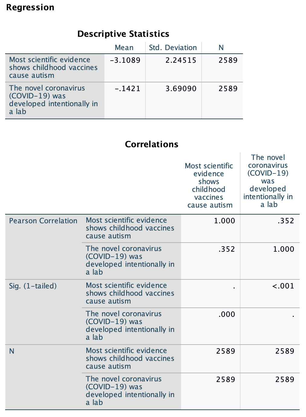
Let's pick up with our Chapter 11 example. In Chapter 11, we looked at whether there was a relationship between people's beliefs about whether COVID-10 was intentionally developed in a lab and whether they thought most scientific evidence shows childhood vaccines cause autism. We determined from the correlation coefficient, Pearson's r, that there was a moderately weak positive relationship (r=0.300). We graphed an equation y=-2.997+0.193x, made predictions based on the equation, and interpreted the slope of the variable as well as whether the relation was significant. We found that, following the 2020 election, on average, the more U.S. eligible voters believed COVID-19 was intentionally developed in a lab, the more likely they were to to believe that most scientific evidence shows childhood vaccines cause autism. However, while confidence levels varied across the independent variable, overall the average respondent, regardless of their belief about whether COVID-19 was intentionally developed in a lab, does not believe that most scientific evidence shows childhood vaccines cause autism.
There are three remaining areas we need to go over:
1. R-Squared, the Coefficient of Determination
Here is the first output we did not interpret in Chapter 11:
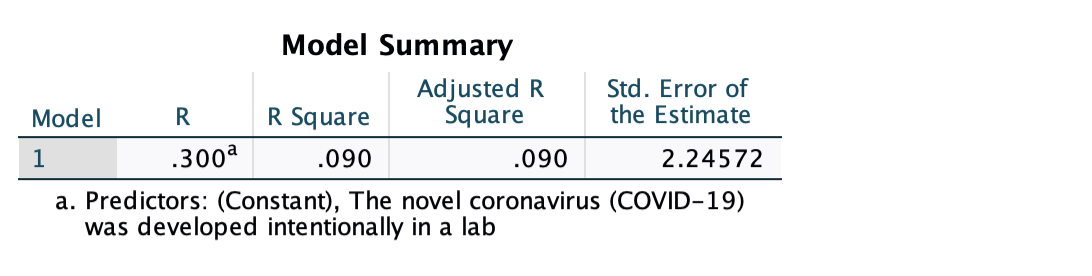
As was noted in Chapter 11, the cell R is the absolute value of Pearson's R, so it gives us strength but not direction. Instead look at the correlation matrix for the correlation value of the bivariate relationship, which gives us both strength and direction. (When we get to multivariate regression, with multiple independent variables, this r value will be the strength for the overall model, so the numbers will be different than the individual bivariate correlations in the correlation matrix.)
The next cell is "R Square."
The coefficient of determination, r2 (r-squared), is the proportion of the dependent variable's variance explained by the independent variable.
R-squared is a "goodness of fit" measure that tells us the independent variable's explanatory power. It is a descriptive sample statistic.
Let's say I was guessing your age. There's a lot of variation in ages. If all I knew was that you were a person in the United States and that the average age in the U.S. is 39.1, my best guess would be that you are 39 years old. However, if I knew something else about you, I may be able to make a more accurate guess. For example, if I knew you were a college student, I'd guess a younger age. Being or not being a college student explains some of the variation in age. It doesn't explain all of it, just some of it. In some cases my prediction would be less accurate. But overall, I can make better predictions of age. If there's a significant relationship between college student status and age, I can make better predictions of your age if I know you are a college student.
Template
[x] explains [r2 x 100] of the variance in [y].
Example
Above, r2=0.090. 0.090x100=9. I am just converting this proportion into a percent.
x, my IV, is belief that COVID-19 was intentionally developed in a lab
y, my DV, is belief that most scientific evidence shows childhood vaccines cause autism
Putting them together:
[x] explains [r2 x 100] of the variance in [y].
Belief that COVID-19 was intentionally developed in a lab explains 9% of the variance in belief that most scientific evidence shows childhood vaccines cause autism.
Other examples:
Physical health explains about one quarter (25.4%) of the variance in mental health).
The percent of a country saying most people can be trusted explains 23.3% of the variance in the percent of a country saying being born in the country is a very important requirement for citizenship.
Where does the r2 value come from?
First, it's lterally r-squared, so for example above r=0.300, so r2=0.300*0.300=0.090, so 9%.
Here is the actual formula for r2:
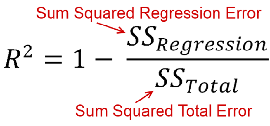
The coefficient of determination is based on explained variation divided by total variation.
Here, the sum of the squared regression error is based on how much each of the points in our scatterplot differ from the line of best fit (squared and summed). Recall that our line of best fit is based on minimizing this statistic. So these residuals are variation from our regression line.
Next, the sum of squared total error ignores the independent variable. It is how much each dependent variable value differs from the mean of the dependent variable (squared and summed) This is variance (standard deviation squared).
The unexplained variance in our regression line divided by the unexplained variance for the dependent variable as a whole gives us the proportion of unexplained variance, the proportion of the dependent variable's variance the independent variable does not explain. We subtract that from 1 to find the proportion of the dependent variable's variance that the independent variable does explain.
To evaluate whether a relationship is substantive, consider r-squared in addition to significance and the 95% confidence interval of the slope. (Or if you are using population data, consider r-squared and the slope.)
2. Overall significance of the model
Here is the second output we did not interpret in Chapter 11:
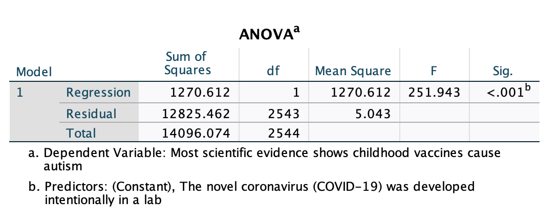
We use the p-value in the cell below "Sig." to evaluate significance for the overall model.
While this is an ANOVA (analysis of variance) test, the p-value should basically match the p-value of our slope in the Coefficients output, since we have a biviarate regression (so the overall model only includes the one independent variable). When we get to multivariate regression with multiple independent variables, these will no longer always match.
The ANOVA F-test here is basically determining the probability that we would draw the sample we did if the r-squared value was actually 0 among our target population. If p<0.05, we are over 95% confident that, among our target population, the independent variable explains more than 0% of the variance in the dependent variable. Recall that when we did a one-way ANOVA test comparing group means we had a between group sum of squares and a within group sum of squares. Here you can see the "regression sum of squares" and "residual sum of squares," concepts discussed above in the r2 behind the scenes.
Null hypothesis: There is no relationship between x and y.
(Statistically, this is that knowing x does not improve prediction of y over just knowing the mean of y.)
Alternative hypothesis: There is a relationship between x and y.
(Statistically, this is that taking x into account improves prediction of y over just knowing the mean of y.)
3. Sample size
Recall that our regression output included descriptives and a correlation matrix:

You can see a few places where N=2545 is listed. This is the weighted sample size, 2,545. Remember that weighting adjusts each case's weight to make the sample better match the target population. However, because of this, the weighted sample size is not the actual number of respondents.
To find the actual sample size, the number of respondents in the sample that we have useable data on for both our independent and dependent variables, we need to find the unweighted sample size. Turn weighting off and then re-run your regression.
Syntax: WEIGHT OFF.
Menu:
Go to Data → Weight Cases. Click "Do not weight cases" and click OK.
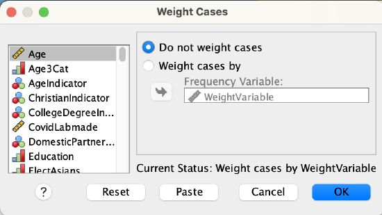
Here's the unweighted output. The unweighted sample size is 2,589. Use the weighted regression for everything else.
The SPSS outputs from regression are not presentation-ready. They have a lot of extra information and the information included is not set up in an easily digestible format. What we'll do here is take the most relevant information and put it into a display table that can be used for your own analysis as well as for communicating to public audiences.
Attached here is a template for bivariate regression display tables. We'll focus on the first template here, the second template below, and the final templates in the document in Chapter 13.
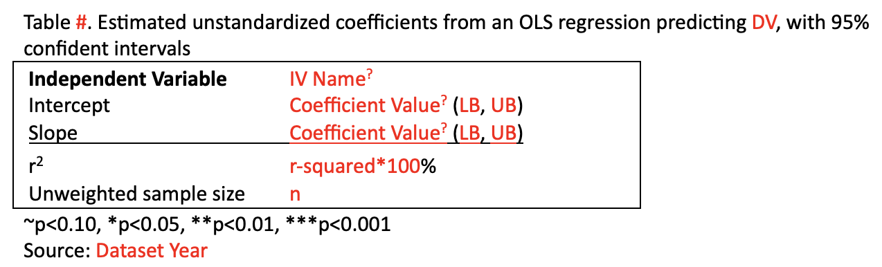
Your job will be to fill out the red parts.
The question mark superscripts are based on your p-values. Next to IV Name you'll use the p-value from the ANOVA output, and then for the intercept and slope you'll use the p-values on those two rows of the coefficients output. Use the key below the table to figure out what symbol to use. If p<0.001, use three asterisks. If p<0.01 but not <0.001, use two asterisks. If p<0.05 but not <0.01, use one asterisk. If p<0.1 but not <0.05, use a tilda. If p≥0.1, do not use any symbol.
LB and UB are for the lower and upper bound of the 95% confidence interval.
In general, I suggest rounding to the nearest hundredths place.
Here's the display table for the regression we've been looking at:
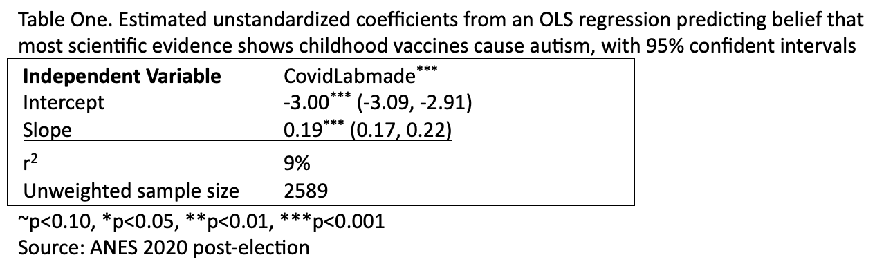
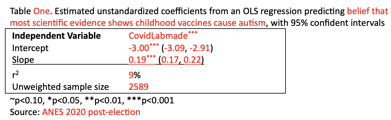 The red parts are what I filled out. Here is the display table without color differentiation:
In order to trust the validity of your OLS regression results, there are some underlying assumptions that must be met. You can read more about these at https://statisticsbyjim.com/regression/ols-linear-regression-assumptions/ and https://statisticsbyjim.com/regression/gauss-markov-theorem-ols-blue/. You will likely need to test that these assumptions are met if you doing a thesis involving regression or trying to pubiish your regression in a scholarly publication.
Bivariate Linear Regression with an Indicator IV
So far we've only looked at bivariate linear regression with a ratio-level or ratio-like independent variable. However, what if you want to include a nominal-level variable (e.g., gender, race, geographic region, religion, etc.) as a predictor? We can also use indicator variables as independent variables for linear regression. Recall that indicator variables are dichotomous variables in which one response is coded as 0 and the other is coded as 1, giving them special properties. You still cannot use them as the dependent variable (for that, you would turn to something called logistic regression). The category coded 0 is the "reference group," the category you are comparing the other to. Sometimes people will name indicator variables with the value for the code of 1 (e.g., Voted, VoteYes, GenderMan, Worried, Midwest, POC). This can help with interpretation.
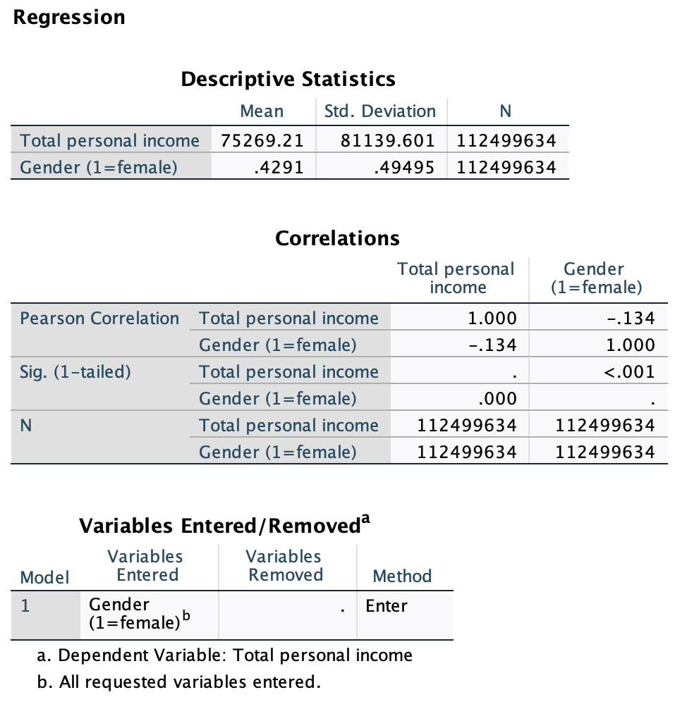
Let's return to our example from earlier in this textbook about the gender pay gap (see Chapter 3 and Chapter 7). Again, we're using 2017 to 2021 American Community Survey data. Our target population below is full-time, year-round, non-institutionalized U.S. workers ages 16+.
SPSS:
There are no differences in running bivariate linear regression when your independent variable is an indicator variable. Just use the indicator variable for your independent variable. However, your independent variable must be coded 0 and 1. In Chapter 7, sex was coded as 1 and 2. In order to use it here for linear regression, I had to re-code it so 0 and 1.
Output:
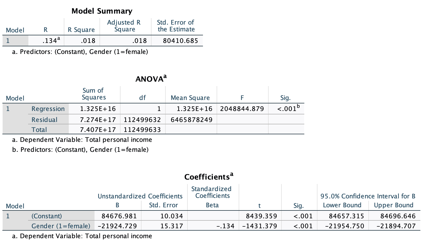
Here is the output from the bivariate linear regression, with gender as the independent variable and income as the dependent variable.
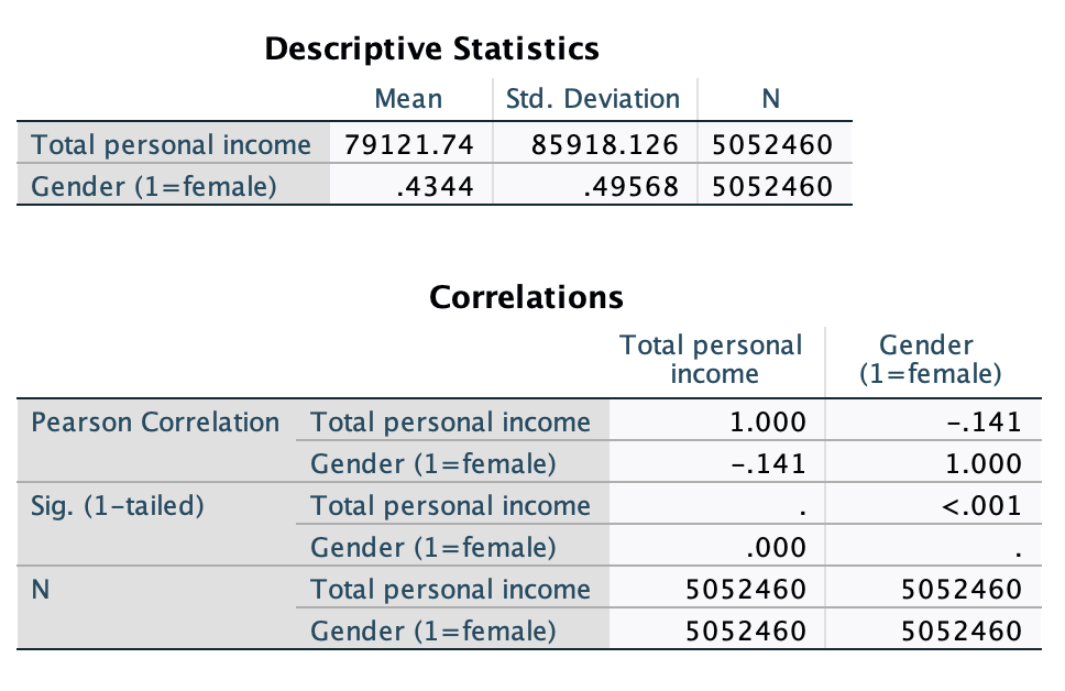
Weighted:
Unweighted:
The display table is almost identical to the one we used above. However, the y-intercept is always interpretable, as it is the predicted value when x=0, and x has meaning at 0 and at 1. Therefore, we add descriptives of what the IV categories are for the intercept and slope.
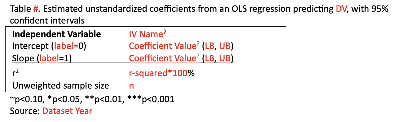
Here's the display table for the regression:
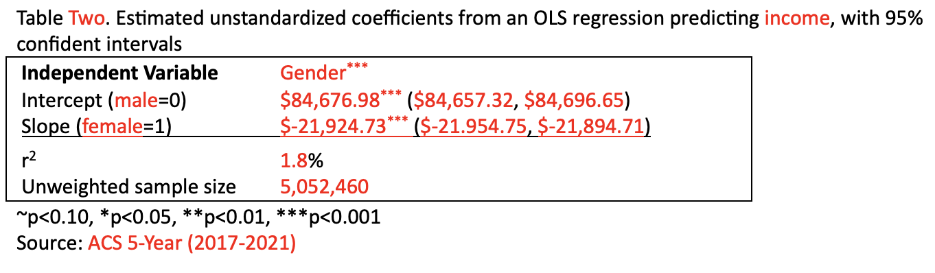
The red parts are what I filled out. Here is the display table without color differentiation:

These interpretations are all the same as before:
We are over 99.9% confident that there is a relationship between gender and income (for 2017 to 2021, among full-time, year-round, non-institutionalized U.S. workers ages 16+).
Here, the intercept, $84,676.98, is the predicted salary estimate for men. We are 95% confident that for all men in the target population, average salary is somewhere between $84,656.32 and $84,696.65.
Gender explains 1.8% of variance in salary.
There were over 5 million people in the sample.
What's Different?
Our interpretation of the slope and our graph will be different.
Here the slope is $-21,924.73. On the one hand, it works the same way. On average, a one unit increase in the IV is associated with a slope-value increase in the DV. Here that means that, on average a one-unit increase in gender is associated with a $21,924.73 decrease in income. However, what is a "one-unit increase in gender"? Based on the coding, this is going from 0 to 1, or from male to female. With the variable being dichotomous, there are no additional unit increases. We also would not typically describe this as an "increase." Instead, we word our interpretation as a comparison between the category coded as 1 and the reference group.
Template: [IV=1 category name]'s average [DV construct name] is predicted to be [slope value] higher than [IV=0 category name] average [DV construct name].
If the slope is negative, share the absolute value for the slope value and change "higher" to "lower."
Example: Women's average income is predicted to be $21,924.73 lower than men's average income.
With a ratio-level or ratio-like independent variable, we make a line graph and the x-axis is a number line. There are many predicted values all along the line.
With an indicator independent variable, x is either 0 or 1. There are only two predicted values. A line graph would inappropriately show movement where there is no x=0.25 or x=0.5 or x=0.75. Therefore, we will use a bar graph.
This Excel template has the graph templates and predicted values worksheets from Chapter 11, but also with a new worksheet, "BivariateGraph.IndicatorIV."
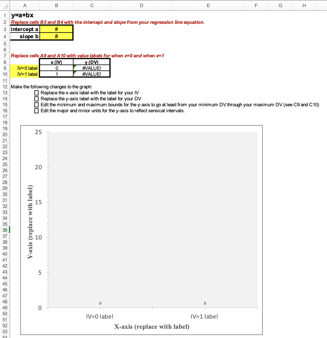
Here you can see I filled in the yellow-shaded cells:
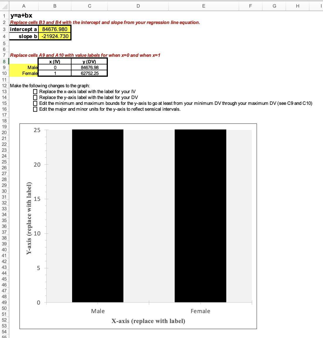
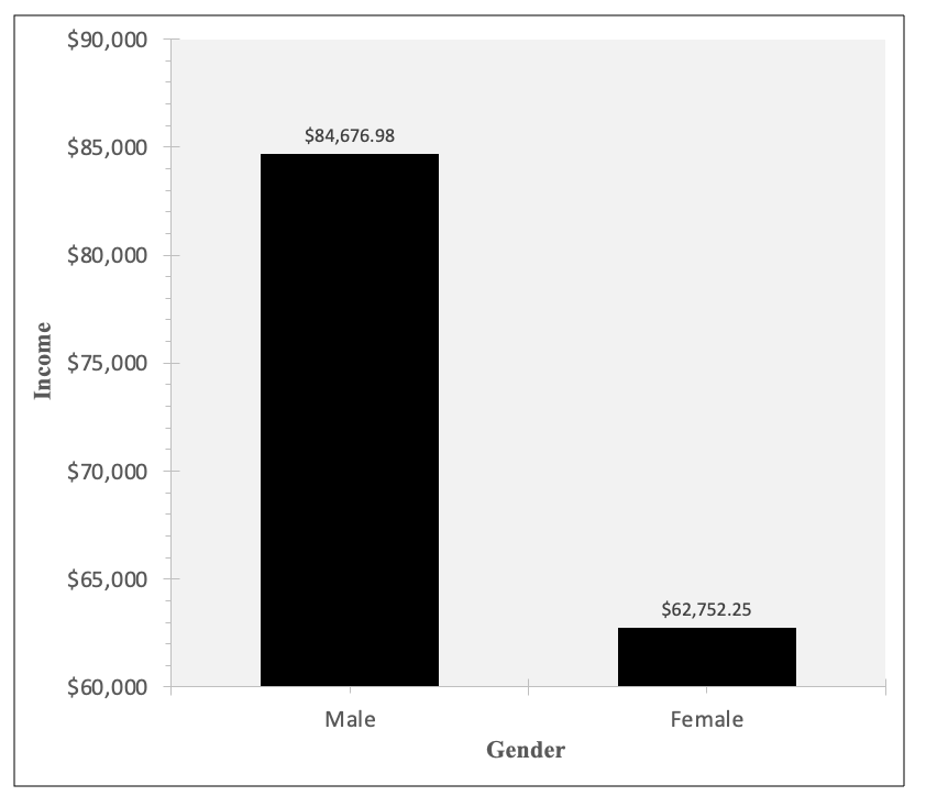
Next I need to edit the x-axis and y-axis labels on the graph, and change the y-axis scale (bounds and units). I also changed the "Number" options to show this as "currency." I don't need to change the x-axis scale, since it is just the two categories, x=0 and x=1, each of which have a bar above them.
Again, it's up to you whether you make the y-axis scale zoom in on the differences or pan out to show the full scale. Here is what both those options look like:

The two-sample t-test we did in Chapter 7 was simpler and gave us the same results:
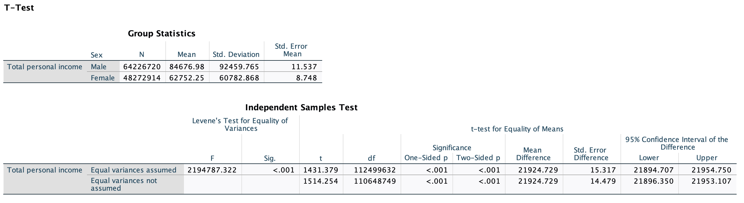
Notice how the means for each group are the same as our predicted values. The p-values match. The mean difference is the same as our slope. If this was the only analysis we were doing, a two-sample t-test would work just as well.
Even if you are doing bivariate regression, you may choose to use regression rather than a two-sample t-test if you are conducting a series of regressions and want to put them all together into one table. If some of your comparisons involve ratio-level independent variables, you cannot use a two-sample t-test for those, but can use regression for all of them and therefore simplify your display table to make it easier to make comparisons.
However, a two-sample t-test is limited to comparing means for one variable (in two groups). Regression is useful because we can do multivariate regression (see Chapter 14), where we have more than one independent variable. If you want to run a regression that includes multiple predictors simultaneously, you need to use regression, not a two-sample t-test.