13: Linear Regression with Reference Group Set Independent Variables
- Page ID
- 191889

\( \newcommand{\vecs}[1]{\overset { \scriptstyle \rightharpoonup} {\mathbf{#1}} } \)
\( \newcommand{\vecd}[1]{\overset{-\!-\!\rightharpoonup}{\vphantom{a}\smash {#1}}} \)
\( \newcommand{\dsum}{\displaystyle\sum\limits} \)
\( \newcommand{\dint}{\displaystyle\int\limits} \)
\( \newcommand{\dlim}{\displaystyle\lim\limits} \)
\( \newcommand{\id}{\mathrm{id}}\) \( \newcommand{\Span}{\mathrm{span}}\)
( \newcommand{\kernel}{\mathrm{null}\,}\) \( \newcommand{\range}{\mathrm{range}\,}\)
\( \newcommand{\RealPart}{\mathrm{Re}}\) \( \newcommand{\ImaginaryPart}{\mathrm{Im}}\)
\( \newcommand{\Argument}{\mathrm{Arg}}\) \( \newcommand{\norm}[1]{\| #1 \|}\)
\( \newcommand{\inner}[2]{\langle #1, #2 \rangle}\)
\( \newcommand{\Span}{\mathrm{span}}\)
\( \newcommand{\id}{\mathrm{id}}\)
\( \newcommand{\Span}{\mathrm{span}}\)
\( \newcommand{\kernel}{\mathrm{null}\,}\)
\( \newcommand{\range}{\mathrm{range}\,}\)
\( \newcommand{\RealPart}{\mathrm{Re}}\)
\( \newcommand{\ImaginaryPart}{\mathrm{Im}}\)
\( \newcommand{\Argument}{\mathrm{Arg}}\)
\( \newcommand{\norm}[1]{\| #1 \|}\)
\( \newcommand{\inner}[2]{\langle #1, #2 \rangle}\)
\( \newcommand{\Span}{\mathrm{span}}\) \( \newcommand{\AA}{\unicode[.8,0]{x212B}}\)
\( \newcommand{\vectorA}[1]{\vec{#1}} % arrow\)
\( \newcommand{\vectorAt}[1]{\vec{\text{#1}}} % arrow\)
\( \newcommand{\vectorB}[1]{\overset { \scriptstyle \rightharpoonup} {\mathbf{#1}} } \)
\( \newcommand{\vectorC}[1]{\textbf{#1}} \)
\( \newcommand{\vectorD}[1]{\overrightarrow{#1}} \)
\( \newcommand{\vectorDt}[1]{\overrightarrow{\text{#1}}} \)
\( \newcommand{\vectE}[1]{\overset{-\!-\!\rightharpoonup}{\vphantom{a}\smash{\mathbf {#1}}}} \)
\( \newcommand{\vecs}[1]{\overset { \scriptstyle \rightharpoonup} {\mathbf{#1}} } \)
\(\newcommand{\longvect}{\overrightarrow}\)
\( \newcommand{\vecd}[1]{\overset{-\!-\!\rightharpoonup}{\vphantom{a}\smash {#1}}} \)
\(\newcommand{\avec}{\mathbf a}\) \(\newcommand{\bvec}{\mathbf b}\) \(\newcommand{\cvec}{\mathbf c}\) \(\newcommand{\dvec}{\mathbf d}\) \(\newcommand{\dtil}{\widetilde{\mathbf d}}\) \(\newcommand{\evec}{\mathbf e}\) \(\newcommand{\fvec}{\mathbf f}\) \(\newcommand{\nvec}{\mathbf n}\) \(\newcommand{\pvec}{\mathbf p}\) \(\newcommand{\qvec}{\mathbf q}\) \(\newcommand{\svec}{\mathbf s}\) \(\newcommand{\tvec}{\mathbf t}\) \(\newcommand{\uvec}{\mathbf u}\) \(\newcommand{\vvec}{\mathbf v}\) \(\newcommand{\wvec}{\mathbf w}\) \(\newcommand{\xvec}{\mathbf x}\) \(\newcommand{\yvec}{\mathbf y}\) \(\newcommand{\zvec}{\mathbf z}\) \(\newcommand{\rvec}{\mathbf r}\) \(\newcommand{\mvec}{\mathbf m}\) \(\newcommand{\zerovec}{\mathbf 0}\) \(\newcommand{\onevec}{\mathbf 1}\) \(\newcommand{\real}{\mathbb R}\) \(\newcommand{\twovec}[2]{\left[\begin{array}{r}#1 \\ #2 \end{array}\right]}\) \(\newcommand{\ctwovec}[2]{\left[\begin{array}{c}#1 \\ #2 \end{array}\right]}\) \(\newcommand{\threevec}[3]{\left[\begin{array}{r}#1 \\ #2 \\ #3 \end{array}\right]}\) \(\newcommand{\cthreevec}[3]{\left[\begin{array}{c}#1 \\ #2 \\ #3 \end{array}\right]}\) \(\newcommand{\fourvec}[4]{\left[\begin{array}{r}#1 \\ #2 \\ #3 \\ #4 \end{array}\right]}\) \(\newcommand{\cfourvec}[4]{\left[\begin{array}{c}#1 \\ #2 \\ #3 \\ #4 \end{array}\right]}\) \(\newcommand{\fivevec}[5]{\left[\begin{array}{r}#1 \\ #2 \\ #3 \\ #4 \\ #5 \\ \end{array}\right]}\) \(\newcommand{\cfivevec}[5]{\left[\begin{array}{c}#1 \\ #2 \\ #3 \\ #4 \\ #5 \\ \end{array}\right]}\) \(\newcommand{\mattwo}[4]{\left[\begin{array}{rr}#1 \amp #2 \\ #3 \amp #4 \\ \end{array}\right]}\) \(\newcommand{\laspan}[1]{\text{Span}\{#1\}}\) \(\newcommand{\bcal}{\cal B}\) \(\newcommand{\ccal}{\cal C}\) \(\newcommand{\scal}{\cal S}\) \(\newcommand{\wcal}{\cal W}\) \(\newcommand{\ecal}{\cal E}\) \(\newcommand{\coords}[2]{\left\{#1\right\}_{#2}}\) \(\newcommand{\gray}[1]{\color{gray}{#1}}\) \(\newcommand{\lgray}[1]{\color{lightgray}{#1}}\) \(\newcommand{\rank}{\operatorname{rank}}\) \(\newcommand{\row}{\text{Row}}\) \(\newcommand{\col}{\text{Col}}\) \(\renewcommand{\row}{\text{Row}}\) \(\newcommand{\nul}{\text{Nul}}\) \(\newcommand{\var}{\text{Var}}\) \(\newcommand{\corr}{\text{corr}}\) \(\newcommand{\len}[1]{\left|#1\right|}\) \(\newcommand{\bbar}{\overline{\bvec}}\) \(\newcommand{\bhat}{\widehat{\bvec}}\) \(\newcommand{\bperp}{\bvec^\perp}\) \(\newcommand{\xhat}{\widehat{\xvec}}\) \(\newcommand{\vhat}{\widehat{\vvec}}\) \(\newcommand{\uhat}{\widehat{\uvec}}\) \(\newcommand{\what}{\widehat{\wvec}}\) \(\newcommand{\Sighat}{\widehat{\Sigma}}\) \(\newcommand{\lt}{<}\) \(\newcommand{\gt}{>}\) \(\newcommand{\amp}{&}\) \(\definecolor{fillinmathshade}{gray}{0.9}\)So far we've covered bivariate linear regression with a ratio-level (or ratio-like) independent variable and with an indicator independent variable. But what if you want to use a nominal variable that has more than two categories? This chapter will show you how to do just that.
Nominal-level variables such as race, geographic region, religion, and marital status cannot be used as is for linear regression. Think back to our scatterplot. The x-axis needs to be ordered to fit the data to a regression line.
However, we already learned that we can use indicator variables (dichotomous variables coded as 0 and 1) as independent variables for linear regression. That's our solution for nominal-level variables as well.
Let's take a variable region with four regions: Northeast, South, Midwest, and West.
One of these regions needs to be the "reference group," which will have the value of 0.
Then we use indicator variables for each of the other categories.
Let's say I choose Northeast as the reference group.
I will then have three indicator variables:
SouthIndicator: 0=Not South (Northeast, Midwest, or West); 1=South
MidwestIndicator: 0=Not Midwest (Northeast, South, or West); 1=Midwest
WestIndicator: 0=Not West (Northeast, South, or Midwest); 1=West
If all three of these variables are zero, then the region is not South, not Midwest, and not West. Since the original region variable only had four options, if all three of these variables are zero, the region is our reference group of Northeast.
This is called a reference group set.
A group of indicator variables for one construct that as a collection represent its various categories. Each category, other than the comparison reference group, has an indicator variable where it is coded as 1.
Remember when we had a variable like gender (as a binary) in Chapter 12 that required one variable? It was coded 0=male, 1=female. Male was the reference group, the category for when the variable was zero. There were two categories, and we needed one variable, one for each category other than the reference group.
When you have nominal-level variables for multiple categories, you have to have indicator variables for each category minus one (each category other than your reference group).
- For example, if your variable was season (Fall, Winter, Spring, Summer), you would designate one season as a reference group (let's do Fall) and then make 3 indicator variables, one for each of the seasons other than Fall.
- For example, if you had a religion variable with: 1) Protestant, 2) Catholic, 3) Muslim, 4) Jewish, 5) Other or multiple religion(s), 6) No religion, you have 6 categories, so would need 5 indicator variables (one for each other than the religion you designate as the reference group).
Let's return to our example from earlier in this textbook about race pay gaps (see Chapter 3 and Chapter 7). Again, we're using 2017 to 2021 American Community Survey data. Our target population below is full-time, year-round, non-institutionalized U.S. workers ages 16+.
We are comparing five racial categories: non-Hispanic White only, non-Hispanic Black only, non-Hispanic Asian-American and Pacific Islander (AAPI); non-Hispanic other or multiracial; Hispanic. My variable Race5Cat has these five mutually exclusive categories.
Let's designate one of these groups as the reference group. I am choosing non-Hispanic (NH) White only. A majority of respondents are NH White only, and this will allow me to compare the pay of other racial groups to Whites.
I don't need a variable for White, because if someone does not fit into any of the other racial groups, that means they are White.
I need a variable for each of the other categories. I started with five racial categories and designated one as my reference group. Therefore I need four indicator variables, one for each of the other categories.
- NH Black only
- NH AAPI only
- NH other/multiracial
- Hispanic
For each of these indicator variables, 0 will be a respondent who is not that category, and 1 will be a repondent who is that category.
- NH Black only (0=Not NH Black only; 1=NH Black only)
- NH AAPI (0=Not NH AAPI only; 1=NH AAPI only)
- NH other/multiracial (0=Not NH other/multiracial; 1=NH other/multiracial)
- Hispanic (0=Not Hispanic; 1=Hispanic)
Each respondent will either have a 0 for all four of these variables if they are NH White only, or a 1 for one of the variables. The coding above is derived from the following:
- NH Black only (0=NH White only, NH AAPI only, NH other/multiracial, or Hispanic; 1=NH Black only)
- NH AAPI (0=NH White only, NH Black only, NH other/multiracial, or Hispanic; 1=NH AAPI only)
- NH other/multiracial (0=NH White only, NH Black only, NH AAPI only, or Hispanic; 1=NH other/multiracial)
- Hispanic (0=NH White only, NH Black only, NH AAPI only, or NH other/multiracial; 1=Hispanic)
Choosing your reference group is based on what you want to compare the other categories to. Usually people choose either the category with the largest sample size or the one that makes sense to compare to others based on their theory/interest/etc.
This is also a technique you can use if you have a ratio-level or ratio-like variable like age or education if they have a relationship with your dependent variable but it's not linear (e.g., it changes direction, or one group is more extremely different than the rest). You can use age groups or degree categories and then make them into a reference group set.
Running the linear regression is almost identical to what we learned in Chapter 11 and did again in Chapter 12, with one difference. Instead of putting in one independent variable, we will put in multiple independent variables --- all the indicator variables that make up the reference group set.
If you mistakenly put in your reference group variable, SPSS will automatically remove one of your IVs from the regression to eliminate redundancy, but it might not be the one you wanted to use as your reference group.
Make sure to only run one bivariate regression, putting all the independent variables that make up the reference group set in together at the same time. You are not running multiple regressions. You want the whole reference group set in at the same time.
Our independent variable, Race5Cat, has 5 racial categories.
There are also 5 indicator variables, one for each category:
- RaceNHWhiteIndicator: NH White only (0=Not NH White only; 1=NH White only)
- RaceNHBlackIndicator: NH Black only (0=Not NH Black only; 1=NH Black only)
- RaceNHAAPIIndicator: NH AAPI (0=Not NH AAPI only; 1=NH AAPI only)
- RaceNHOtherIndicator: NH other/multiracial (0=Not NH other/multiracial; 1=NH other/multiracial)
- RaceHispanicIndicator: Hispanic (0=Not Hispanic; 1=Hispanic)
I can't use Race5Cat as an IV for linear regression, because it's nominal.
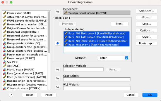
I designate one of the five categories as the reference group. In this case, I chose NH White only. Therefore, RaceNHWhiteIndicator will not go into my regression. If all the other four variables have a value of 0, that indicates the respondent is NH White only.
The other four variable constitute my reference group set and will all go into my regression. Therefore, I have four IVs to put in: RaceNHBlackIndicator, RaceNHAAPIIndicator, RaceNHOtherIndicator, and RaceHispanicIndicator.
Syntax:
The difference in syntax is with the line:
/METHOD=ENTER IVName.
Instead of entering the name of one independent variable, you will enter however many variables make up your reference group set (total number of categories minus the reference group), with a space in between each.
/METHOD=ENTER IV1Name IV2Name IV3Name IV4Name.
/METHOD=ENTER RaceNHBlackIndicator RaceNHAAPIIndicator RaceNHOtherIndicator RaceHispanicIndicator.
The full syntax therefore looks like this:
REGRESSION
/DESCRIPTIVES MEAN STDDEV CORR SIG N
/MISSING LISTWISE
/STATISTICS COEFF OUTS CI(95) R ANOVA
/CRITERIA=PIN(.05) POUT(.10) TOLERANCE(.0001)
/NOORIGIN
/DEPENDENT DVName
/METHOD=ENTER IV1Name IV2Name IV3Name IV4Name.
Menu:
Previously you put your independent variable in the “Independent(s)” box and your dependent variable in the “Dependent” box.
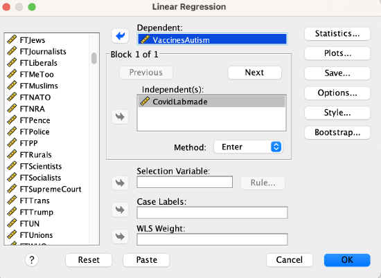
The only change is that you will put all of the independent variables that constitute your reference group set (one indicator variable for each category except for the reference group) into the "Independent(s):" box.
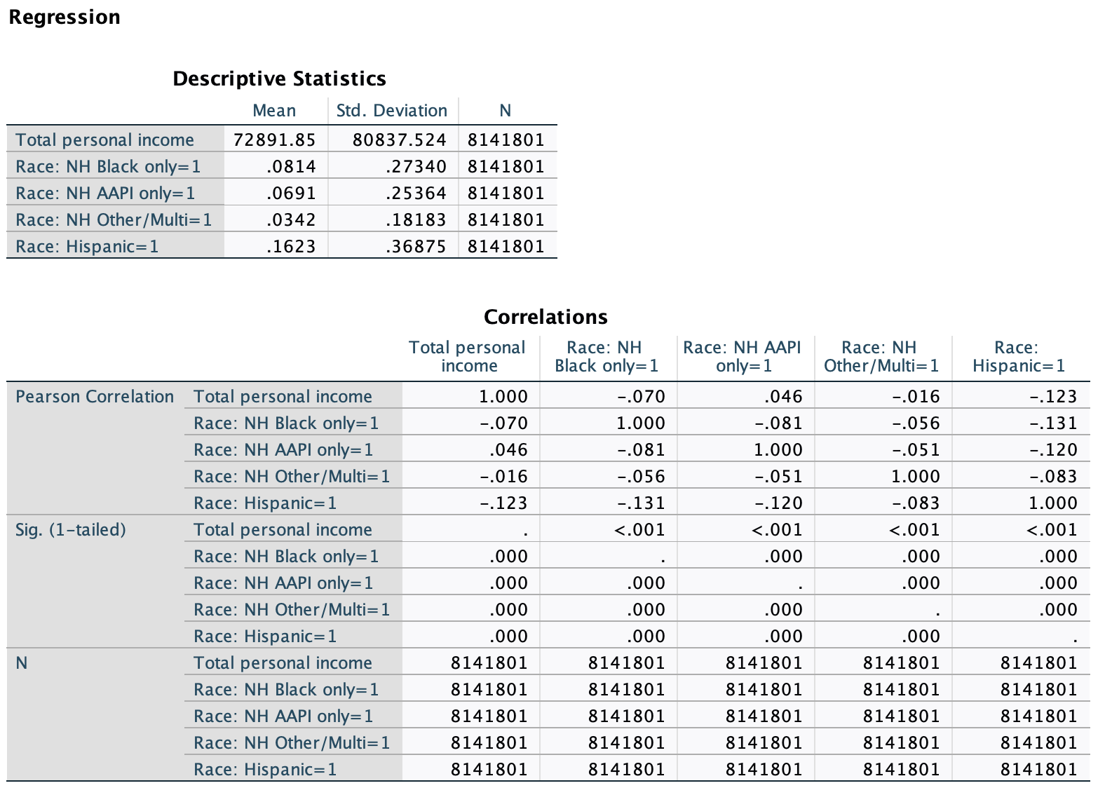
SPSS Output
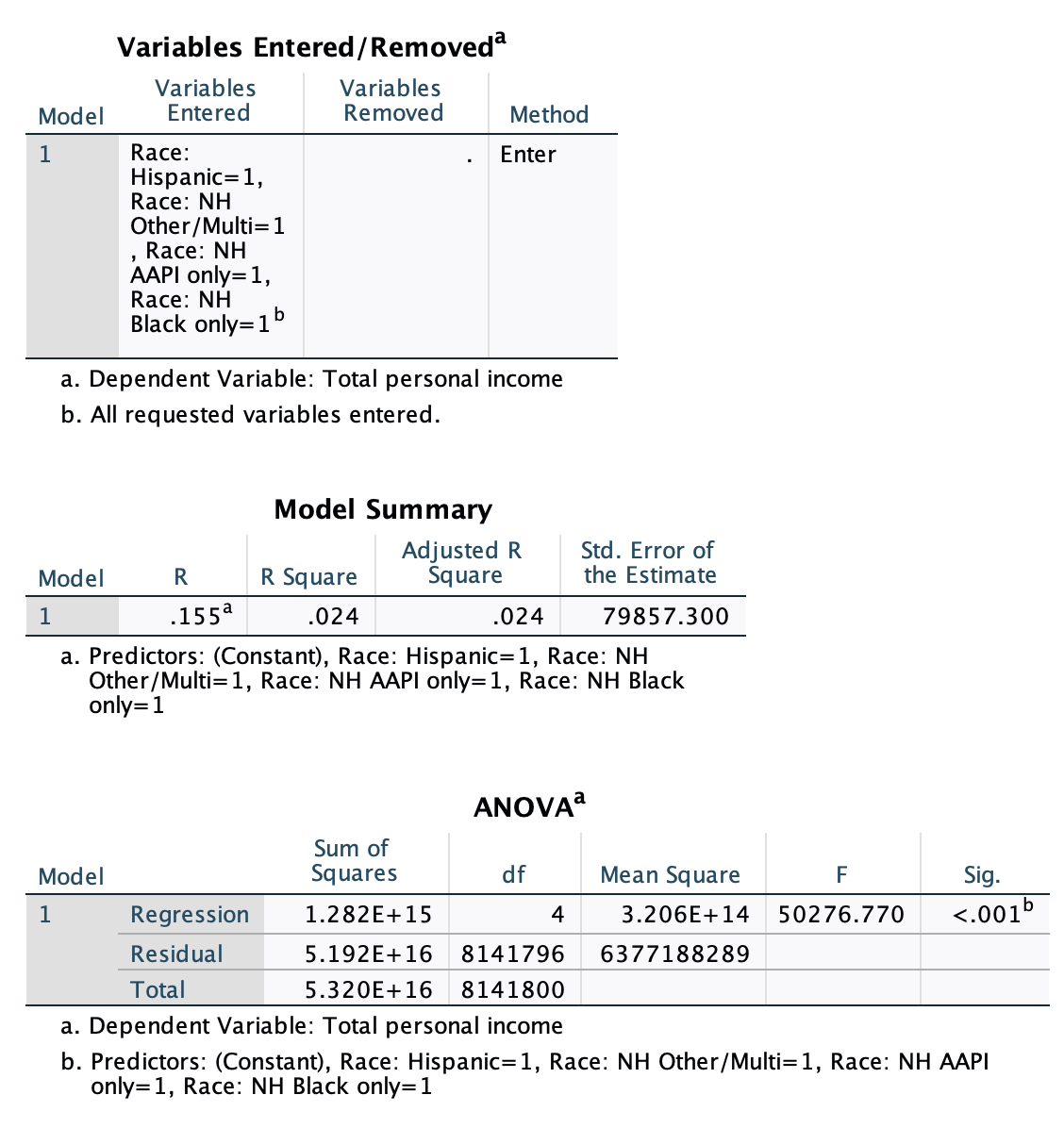
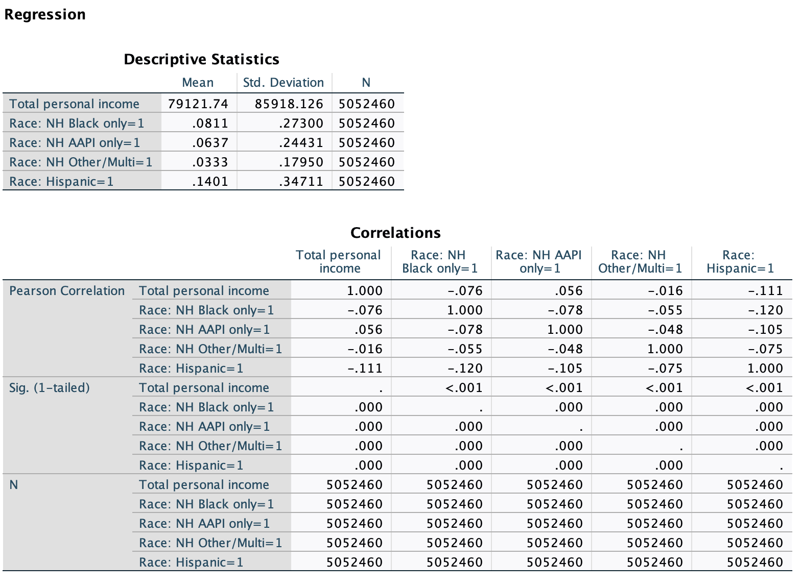
The output looks similar to what we had before, except that the coefficients output has more rows. Beyond the y-intercept row, there is one for each independent variable's slope. There are also more variables and correlation pairs in the descriptive statistics and correlations outputs. The correlation coefficient (Pearson's r) in the model summary output may not match the (absolute value of the) individual correlation values in the Correlations output, as the model summary is taking into account all the reference group set variables collectively to determine the strength of the relationship, rather than just one indicator variable on its own. Finally, the p-value in the ANOVA output may not be the same as p-values in the coefficients output, as the ANOVA output p-value is for the model as a whole, the whole construct of the reference group set collectively, whereas the p-values in the coefficients output are about whether each individual category's predicted dependent variable value is significantly different from the reference group (with the y-intercept p-value still evaluating confidence in whether the predicted dependent variable value for the reference group category is different from zero).


Unweighted:
The display tables template from Chapter 12 BivariateOLSLinearRegression.DisplayTableTemplates.docx has three templates for bivariate linear regression with a reference group set for the independent variable(s).
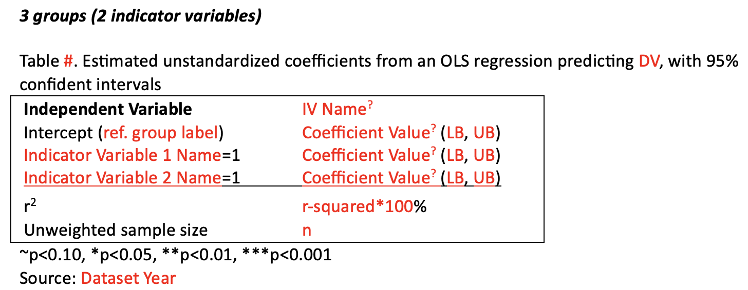
The first template is for if your independent variable construct has three groups and you therefore put two indicator variables into your regression. For example, if you were using gender as your independent variable with man, woman, and genderqueer as the three categories, you would use this template:
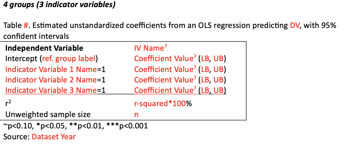
The second template is for if your variable has four categories, and you therefore put in three indicator variables (with the fourth category serving as your reference group).
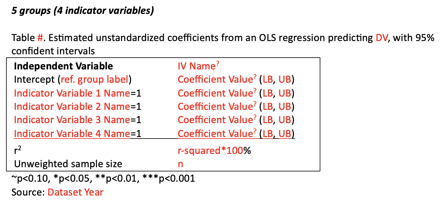
The third template is for if your variable has five categories, and you therefore put in four indicator variables.
If you have more than five categories, you may want to consider collapsing categories together so that you have fewer categories. If you have good reason to have more than five discrete categories, you will need to add another row to the template yourself.
With the race pay gap example, we had five racial groups and put in four independent variables (with NH White only serving as our reference group), so I will use the template for "5 groups (4 indicator variables)."
I edited the summary display table below for everything that is in red:
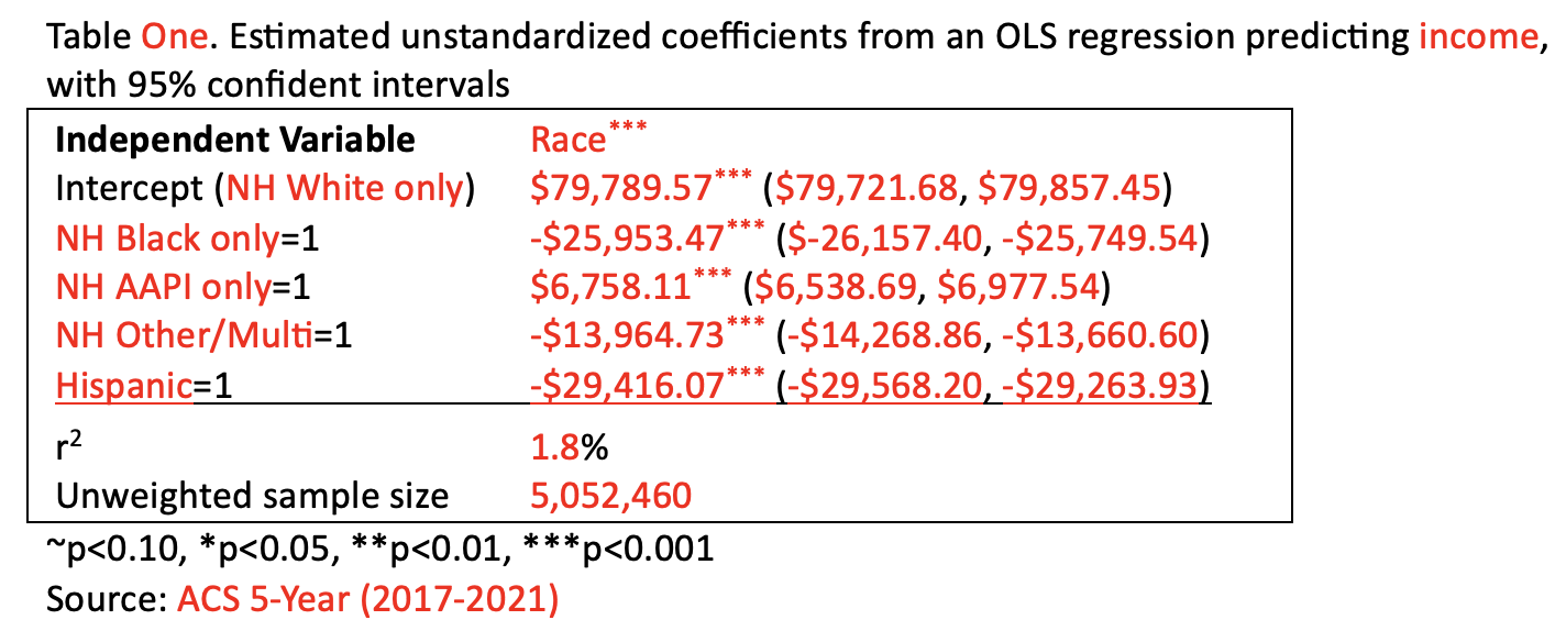
Here is the display table with all of it in black:
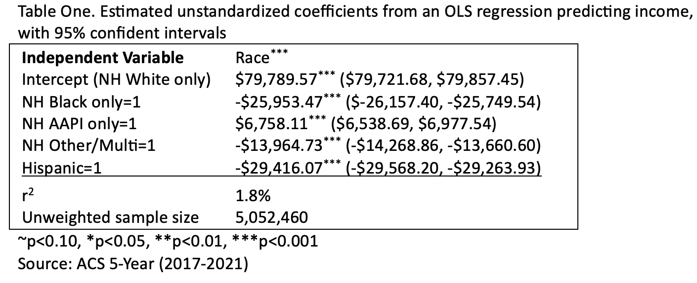
The r-squared value is for the model as a whole, so not for the explained variance from any one category, but from all of them together, collectively. Here, this means that race explains 1.8% of variance in income.
For this example, all of the p-values were <0.001, both weighted and unweighted. This may be because there are over 5 million cases in the sample. The *** after Race is the p-value from the ANOVA output and signifies whether race as a whole is has a significant relationship with income among our target population. The other *** come from the Coefficients output. I'll briefly show you an example at the end of the chapter that has p-values that are not all identical.
The interpretation of the y-intercept and slopes will mirror our interpretation from Chapter 12 where we used one indicator variable as the independent variable. Each slope is in comparison to the reference group. The p-values are the probability that we would pull this sample if the slope was actually zero, meaning if there was no difference between this category's predicted dependent variable value and the reference group's predicted dependent variable value.
Here is the coefficients output from our race pay gap linear regression.
NH White only
- The first row, constant, is for the y-intercept. When all the other variables (NH Black Only, NH AAPI only, NH Other/Multi, and Hispanic) are zero, then we are left with our reference group, in this case NH White only.
- The value in the unstandardized coefficients B cell for the Constant row, $79,789.57, is the predicted income (years 2017 to 2021) for NH White only full-time, year-round, non-institutionalized U.S. workers ages 16+. This predicted value is based on the sample.
- For the target population, we can look at the confidence interval. We are 95% confident that the average income for this group is somewhere between $79,721.68 and $79,857.45.
- The p-value, p<0.001, means that we are over 99.9% confident that the sample coefficient, $79,789.57, is not actually $0 for our target population. This makes sense --- the average salary for NH white only full-time U.S. adult workers should not be $0. The p-value for the y-intercept does not tell us anything about whether or not there is a relationship between race and income.
NH Black only
- The second row, RaceNHBlackIndicator, is for our indicator variable for the NH Black only category.
- The value in the unstandardized coefficients B cell for this row, -$25,953.47, is a sample statistic comparing the average income for NH Black only respondents to the average income for the reference group, in this case NH White only respondents. NH Black only respondents are predicted to have an income $25,953.47 less than NH White only respondents.
- Since NH White only respondents are predicted to have an average income of $79,789.57, we can also calculate the predicted income for NH Black only respondents: $79,789.57-$25,953.47=$53,836.10.
- The slope and the predicted value here are based on the sample. For the target population, we can look at the confidence interval. We are 95% confident that among all NH Black only workers (full-time, year-round, non-institutionalized U.S. workers ages 16+ from 2017 to 2021), they have, on average, an income somewhere between $25,749.54 and $26,157.40 less than their NH White only worker counterparts.
- The p-value indicates the probability that we would pull this sample if this slope were actually zero. Again, the slope is comparing this category to the reference group. So the p-value is indicating whether there is a significant difference between this category's predicted income and the reference group's predicted income. With p<0.001, we are over 99.9% confident that there is a difference between NH Black only workers' average income and NH White only workers' average income among our target population (full-time, year-round, non-institutionalized U.S. workers ages 16+ from 2017 to 2021).
NH AAPI only
- The third row is for our NH AAPI only category.
- The slope, $6,758.11, means that among our respondents, the average income for NH AAPI only workers is $6,758.11 higher than the average income for NH White only workers.
- Our predicted income for NH AAPI only respondents, $79,789.57+$6,758.11, is $86,547.68.
- The confidence interval indicates that we are 95% confident that, among all workers in this target population, the average income for NH AAPI workers is somewhere between $6,538.69 and $6,977.54 higher than the average income for NH White only workers.
- The p-value indicates that we are over 99.9% confident, that among our target population (full-time, year-round, non-institutionalized U.S. workers ages 16+ from 2017 to 2021), NH AAPI only and NH White only workers have a different average income.
NH Other/Multiracial
- The fourth row is for our NH other race or multiracial category.
- The slope, -$13,964.73, means that among our respondents, the average income for NH other/multiracial workers is $13,964.73 lower than the average income for NH White only workers.
- Our predicted income for NH other/multiracial respondents, $79,789.57+(-$13,964.73), is $65,824.84.
- The confidence interval indicates that we are 95% confident that, among all workers in this target population, the average income for NH other/multiracial workers is somewhere between $13,660.60 and $14,268.86 lower than the average income for NH White only workers.
- The p-value indicates that we are over 99.9% confident, that among our target population (full-time, year-round, non-institutionalized U.S. workers ages 16+ from 2017 to 2021), NH other/multiracial and NH White only workers have a different average income.
Hispanic
- The fifth row is for our Hispanic category.
- The slope, -$29,416.07, means that among our respondents, the average income for Hispanic workers is $29,416.07 lower than the average income for NH White only workers.
- Our predicted income for Hispanic respondents, $79,789.57+(-$29,416.07), is $50,373.50.
- The confidence interval indicates that we are 95% confident that, among all workers in this target population, the average income for Hispanic workers is somewhere between $29,263.93 and $29,568.20 lower than the average income for NH White only workers.
- The p-value indicates that we are over 99.9% confident, that among our target population (full-time, year-round, non-institutionalized U.S. workers ages 16+ from 2017 to 2021), Hispanic and NH White only workers have a different average income.
The slopes, p-values, and confidence intervals for each of the variables is only for that category in relation to the reference group. If you want to compare two categories to each other to see if they are significantly different, you would need to figure this out using the confidence intervals of the slopes for each of those categories' predicted values and determine whether the confidence intervals of their predicted values would overlap.
Regression Equation
Previously our regression equation was y=a+bx, where y is the dependent variable, a is the y-intercept, b is the slope, and x is the independent variable.
Now we have more than one independent variable, so we need to extend this equation.
If there are two independent variables, our equation will be: y=a+b1x1+b2x2, where x1 is the first independent variable, b1 the slope for that variable, x2 the second independent variable, and b2 the slope for that second variable.
If there are three independent variables, our equation will be: y=a+b1x1+b2x2+b3x3.
If there are four independent variables, our equation will be: y=a+b1x1+b2x2+b3x3+b4x4.
And so forth.
You don't have to use x1, x2, x3, etc. for your notation. I prefer to use a letter that lets me know what the category is. For example, if I were using region with Northeast as my reference group set and three indicator variables: SouthIndicator, MidwestIndicator, and WestIndicator, I might use S for South, M for Midwest, and W for West. My equation would be y=a+bSS+bMM+bWW, or y=a+b1S+b2M+b3W is fine as well. I could also write it without the subscripts for the slopes as long as I know that they are not all the same, and with words for the variables, e.g., y=a+b(South)+b(Midwest)+b(West). Just stay away from abbreviating variables into two letters; for example, I would not want to use MW for midwest (y=a+bSS+bMWMW+bWW) because this would be confusing as to whether MW is for the midwest or for a variable M multipled by a variable W.
My equation will look like: y=a+b1x1+b2x2+b3x3+b4x4.
I am going to use letters for each variable: B for NH Black only, A for NH AAPI only, O for NH other/multi, and H for Hispanic.
Therefore my equation will look like: y=a+b1B+b2A+b3O+b4H.
Filling in the coefficients, my equation is: y = $79,789.57 + -$25,953.47(B) + $6,758.11(A) + -$13,964.73(O) + -$29,416.07(H).
Again, I could also write this as: y = $79,789.57 + -$25,953.47(Black) + $6,758.11(Aapi) + -$13,964.73(Other) + -$29,416.07(Hispanic), or as
y = $79,789.57 + -$25,953.47(x1) + $6,758.11(x2) + -$13,964.73(x3) + -$29,416.07(x4).
Only write one equation for the entire regression, and put all the coefficients and variables into the one equation. Do not write multiple equations for different variables.
Making Predictions
Just like before, I can make predictions by plugging variable values into the equation and solving for y.
y = $79,789.57 + -$25,953.47(B) + $6,758.11(A) + -$13,964.73(O) + -$29,416.07(H).
Prediction for NH White only
Black=0, AAPI=0, Other/Multi=0, Hispanic=0
y = $79,789.57 + -$25,953.47(0) + $6,758.11(0) + -$13,964.73(0) + -$29,416.07(0)
y = $79,789.57 + 0 + 0 + 0 + 0
y = $79,789.57
Prediction for NH Black only
Black=1, AAPI=0, Other/Multi=0, Hispanic=0
y = $79,789.57 + -$25,953.47(1) + $6,758.11(0) + -$13,964.73(0) + -$29,416.07(0)
y = $79,789.57 + (-$25,953.47) + 0 + 0 + 0
y = $53,836.10
Prediction for NH AAPI only
Black=0, AAPI=1, Other/Multi=0, Hispanic=0
y = $79,789.57 + -$25,953.47(0) + $6,758.11(1) + -$13,964.73(0) + -$29,416.07(0)
y = $79,789.57 + 0 + $6,758.11 + 0 + 0
y = $86,547.68
Prediction for NH Other/Multi
Black=0, AAPI=0, Other/Multi=1, Hispanic=0
y = $79,789.57 + -$25,953.47(0) + $6,758.11(0) + -$13,964.73(1) + -$29,416.07(0)
y = $79,789.57 + 0 + 0 + (-$13,964.73) + 0
y = $65,824.84
Prediction for Hispanic
Black=0, AAPI=0, Other/Multi=0, Hispanic=1
y = $79,789.57 + -$25,953.47(0) + $6,758.11(0) + -$13,964.73(0) + -$29,416.07(1)
y = $79,789.57 + 0 + 0 + 0 + (-$29,416.07)
y = $50,373.50
Because, with a reference group set, all the variables are 0 or one of the variables is 1 and the rest are 0, I can also just use the y-intercept and slope for the category I'm interested in, and ignore the rest of the equation (which will be zero). The reference group category's predicted value is the y-intercept, and any other category's predicted value is the y-intercept plus the slope for that category.
y-intercept: $79,789.57
NH Black only slope: -$25,953.47
NH AAPI only slope: $6,758.11
NH Other/Multiracial slope: -$13,964.73
NH Hispanic slope: -$29,416.07
Prediction for NH White only
y-intercept = $79,789.57
Prediction for NH Black only
y-intercept + Black slope
y = $79,789.57 + (-$25,953.47) = $53,836.10
Prediction for NH AAPI only
y-intercept + AAPI slope
y = $79,789.57 + $6,758.11 = $86,547.68
Prediction for NH Other/Multi
y-intercept + Other/Multi slope
y = $79,789.57 + (-$13,964.73) = $65,824.84
Prediction for Hispanic
y-intercept + Hispanic slope
y = $79,789.57 + (-$29,416.07) = $50,373.50
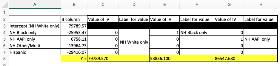
I have added an additional worksheet to the BivariateLinearRegressionGraphTemplate.xlsx that you can use for calculating predicted values when you have multiple independent variables (see worksheet labeled PredictedValueCalc.MultipleIVs).
Because we are using a reference group set that came from an original variable with mutually exclusive categories, just make sure that either all the variables are zero if you are predicting the reference group category, or that only one IV has a value of 1 and the rest have a value of 0, with the value of 1 for the category you are making the prediction for.
Here is the worksheet filled out for the first three categories.
Just like when we had only one indicator variable, we cannot make a line graph to graph out the equation. Each independent variable value is either 0 or 1. The independent variable construct is categorical. So instead, we make a bar graph. While last chapter our bar graph had two bars, one for each category, here we will have multiple bars, with bars for however many categories your construct has.
The graphing template in Excel: BivariateLinearRegressionGraphTemplate.xlsx, has three worksheets for this. BivariateGraph.3CatIV is for if you have three categories, BivariateGraph.4CatIV is if you have four categories, and BivariateGraph.5CatIV is for if you have five categories. If you have more than five categories you may want to consider collapsing categories together, but otherwise you will need to edit the template yourself.
The template works the same as before, except you have to add in additional slopes and category descriptions, for your y-intercept and then one for each of your independent variables.
I am using the graphing template for 5 categories.
Here is the template with the yellow squares filed out:

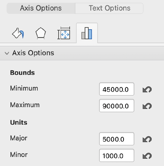
Next I had to replace the x-axis and y-axis labels on my graph and edit the bounds and units for the y-axis. I can tell from cells C12 through C16 above that the dependent variable values range from just over $50,000 to just under $87,000. Here is what I put in for bounds and units:
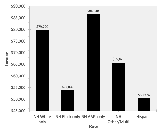
Here is the graph I ended up with:
The one-way ANOVA (with confidence intervals) we did in Chapter 7 was simpler and gave us the same overall p-value and more accurate sample group means:

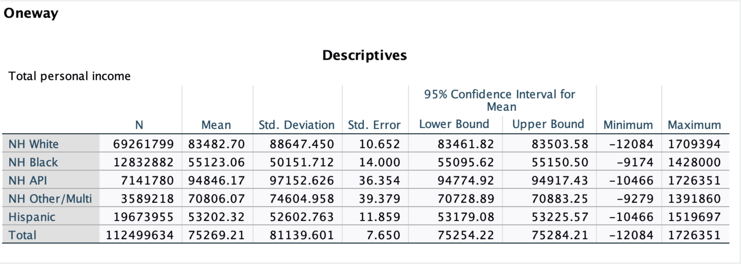
If the only analysis we were doing was race by income, a one-way ANOVA test would work just as well.
Even if you are doing bivariate regression, you may choose to use regression rather than ANOVA if you are conducting a series of regressions and want to put them all together into one table. If some of your comparisons involve ratio-level independent variables, you cannot use a one-way ANOVA for those, but can use regression for all of them and therefore simplify your display table to make it easier to make comparisons.
However, a one-way ANOVA is limited to comparing means for one variable (in multiple categorical groups). Regression is useful because we can do multivariate regression (see Chapter 14), where we have more than one independent variable construct. If you want to run a regression that includes multiple predictors simultaneously, you need to use regression, not a one-way ANOVA.
Let's look at one more example, briefly. This example uses the American National Election Studies post-2020 election dataset. The target population is U.S. eligible voters.
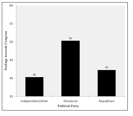
Here my dependent variable is feelings towards Congress, on a 0 to 100 scale, with 0 degrees being cold, 50 degrees neutral, and 100 degrees warm.
For my independent variable, I am using political party, in three categories: Democratic, Independent/other party, and Republican. I chose Independent/other party as my reference group, so I am left with two indicator variables to put in: one for Democratic=1 and one for Republican=1.
Here is some of the output from the linear regression:
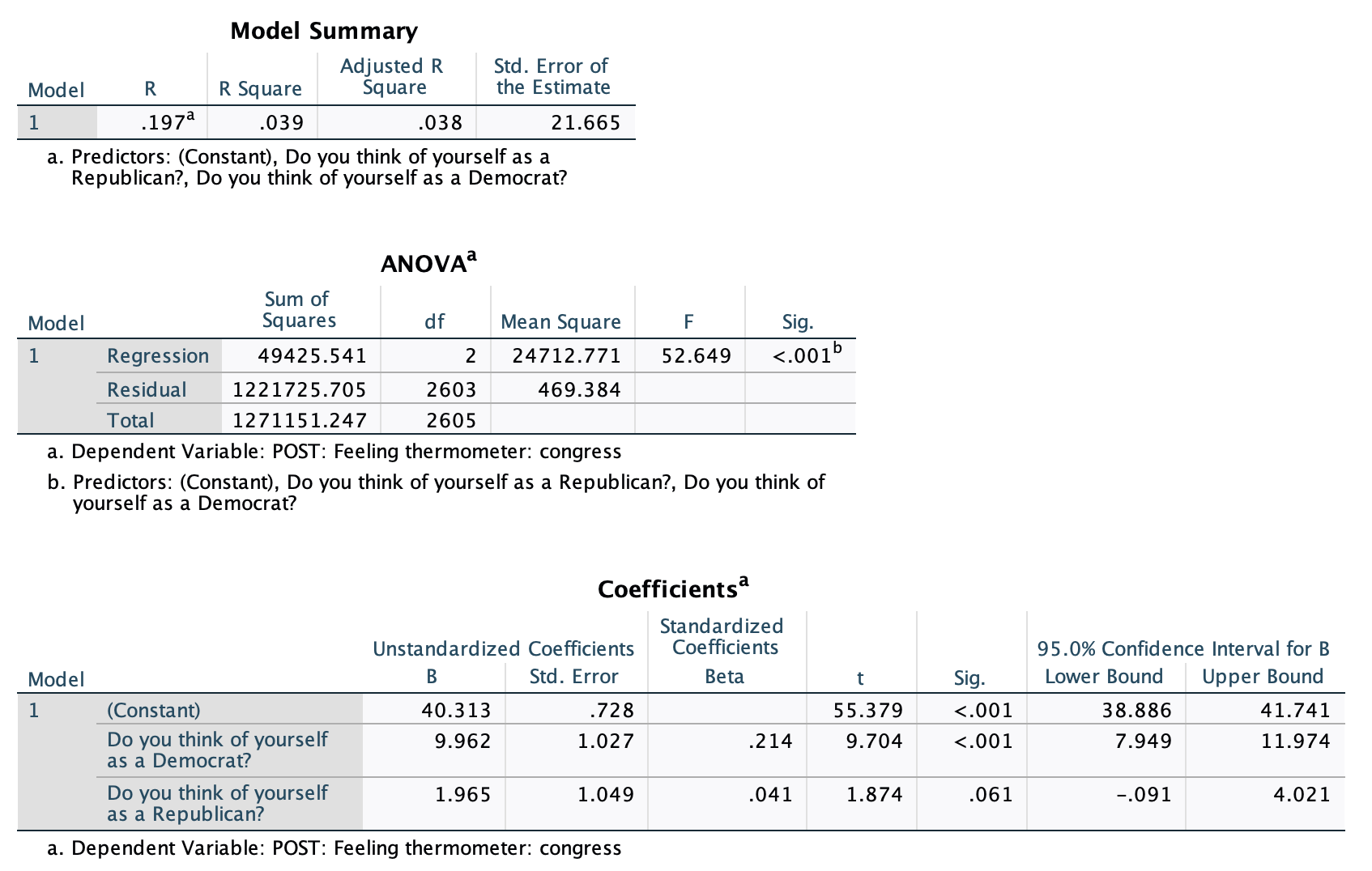
Overall, based on the p-value in the ANOVA output, I am over 99.9% confident that political party has a significant relationship with feelings towards Congress (over 99.9% confident that the relationship exists among eligible voters following the 2020 election).
Based on my r-squared value, political party explains 3.9% of variance in feelings towards Congress.
When I get to my coefficients output, I can see that my p-values do not all match the p-value from the ANOVA output. The ANOVA output p-value is telling me whether collectively political party has a relationship with feelings towards Congress (the probability I would pull this sample if r-squared, the explained variance, is actually zero). In the coefficients output, the p-values for the Democrat and Republican rows are for whether these are significantly different from the reference group. We are over 99.9% confident that Democrats (who are eligible voters, following the 2020 election) have different feelings towards Congress than Independents/Other. We are 93.9% confident that Republicans (who are eligible voters, following the 2020 election) have different feelings towards Congress than Independents/Other. There is a significant difference between Democrats and Independents/other. There is not a significant different (or there is a marginally significant difference, p<0.1 but not <0.05) between Republicans and Independents/other. If I made a summary display table for this regression, the independent variable construct at the top would have ***, and then below Democrat would have ***, while GOP would be marked with ~.