14: Multivariate Linear Regression
- Page ID
- 194404
\( \newcommand{\vecs}[1]{\overset { \scriptstyle \rightharpoonup} {\mathbf{#1}} } \)
\( \newcommand{\vecd}[1]{\overset{-\!-\!\rightharpoonup}{\vphantom{a}\smash {#1}}} \)
\( \newcommand{\dsum}{\displaystyle\sum\limits} \)
\( \newcommand{\dint}{\displaystyle\int\limits} \)
\( \newcommand{\dlim}{\displaystyle\lim\limits} \)
\( \newcommand{\id}{\mathrm{id}}\) \( \newcommand{\Span}{\mathrm{span}}\)
( \newcommand{\kernel}{\mathrm{null}\,}\) \( \newcommand{\range}{\mathrm{range}\,}\)
\( \newcommand{\RealPart}{\mathrm{Re}}\) \( \newcommand{\ImaginaryPart}{\mathrm{Im}}\)
\( \newcommand{\Argument}{\mathrm{Arg}}\) \( \newcommand{\norm}[1]{\| #1 \|}\)
\( \newcommand{\inner}[2]{\langle #1, #2 \rangle}\)
\( \newcommand{\Span}{\mathrm{span}}\)
\( \newcommand{\id}{\mathrm{id}}\)
\( \newcommand{\Span}{\mathrm{span}}\)
\( \newcommand{\kernel}{\mathrm{null}\,}\)
\( \newcommand{\range}{\mathrm{range}\,}\)
\( \newcommand{\RealPart}{\mathrm{Re}}\)
\( \newcommand{\ImaginaryPart}{\mathrm{Im}}\)
\( \newcommand{\Argument}{\mathrm{Arg}}\)
\( \newcommand{\norm}[1]{\| #1 \|}\)
\( \newcommand{\inner}[2]{\langle #1, #2 \rangle}\)
\( \newcommand{\Span}{\mathrm{span}}\) \( \newcommand{\AA}{\unicode[.8,0]{x212B}}\)
\( \newcommand{\vectorA}[1]{\vec{#1}} % arrow\)
\( \newcommand{\vectorAt}[1]{\vec{\text{#1}}} % arrow\)
\( \newcommand{\vectorB}[1]{\overset { \scriptstyle \rightharpoonup} {\mathbf{#1}} } \)
\( \newcommand{\vectorC}[1]{\textbf{#1}} \)
\( \newcommand{\vectorD}[1]{\overrightarrow{#1}} \)
\( \newcommand{\vectorDt}[1]{\overrightarrow{\text{#1}}} \)
\( \newcommand{\vectE}[1]{\overset{-\!-\!\rightharpoonup}{\vphantom{a}\smash{\mathbf {#1}}}} \)
\( \newcommand{\vecs}[1]{\overset { \scriptstyle \rightharpoonup} {\mathbf{#1}} } \)
\( \newcommand{\vecd}[1]{\overset{-\!-\!\rightharpoonup}{\vphantom{a}\smash {#1}}} \)
\(\newcommand{\avec}{\mathbf a}\) \(\newcommand{\bvec}{\mathbf b}\) \(\newcommand{\cvec}{\mathbf c}\) \(\newcommand{\dvec}{\mathbf d}\) \(\newcommand{\dtil}{\widetilde{\mathbf d}}\) \(\newcommand{\evec}{\mathbf e}\) \(\newcommand{\fvec}{\mathbf f}\) \(\newcommand{\nvec}{\mathbf n}\) \(\newcommand{\pvec}{\mathbf p}\) \(\newcommand{\qvec}{\mathbf q}\) \(\newcommand{\svec}{\mathbf s}\) \(\newcommand{\tvec}{\mathbf t}\) \(\newcommand{\uvec}{\mathbf u}\) \(\newcommand{\vvec}{\mathbf v}\) \(\newcommand{\wvec}{\mathbf w}\) \(\newcommand{\xvec}{\mathbf x}\) \(\newcommand{\yvec}{\mathbf y}\) \(\newcommand{\zvec}{\mathbf z}\) \(\newcommand{\rvec}{\mathbf r}\) \(\newcommand{\mvec}{\mathbf m}\) \(\newcommand{\zerovec}{\mathbf 0}\) \(\newcommand{\onevec}{\mathbf 1}\) \(\newcommand{\real}{\mathbb R}\) \(\newcommand{\twovec}[2]{\left[\begin{array}{r}#1 \\ #2 \end{array}\right]}\) \(\newcommand{\ctwovec}[2]{\left[\begin{array}{c}#1 \\ #2 \end{array}\right]}\) \(\newcommand{\threevec}[3]{\left[\begin{array}{r}#1 \\ #2 \\ #3 \end{array}\right]}\) \(\newcommand{\cthreevec}[3]{\left[\begin{array}{c}#1 \\ #2 \\ #3 \end{array}\right]}\) \(\newcommand{\fourvec}[4]{\left[\begin{array}{r}#1 \\ #2 \\ #3 \\ #4 \end{array}\right]}\) \(\newcommand{\cfourvec}[4]{\left[\begin{array}{c}#1 \\ #2 \\ #3 \\ #4 \end{array}\right]}\) \(\newcommand{\fivevec}[5]{\left[\begin{array}{r}#1 \\ #2 \\ #3 \\ #4 \\ #5 \\ \end{array}\right]}\) \(\newcommand{\cfivevec}[5]{\left[\begin{array}{c}#1 \\ #2 \\ #3 \\ #4 \\ #5 \\ \end{array}\right]}\) \(\newcommand{\mattwo}[4]{\left[\begin{array}{rr}#1 \amp #2 \\ #3 \amp #4 \\ \end{array}\right]}\) \(\newcommand{\laspan}[1]{\text{Span}\{#1\}}\) \(\newcommand{\bcal}{\cal B}\) \(\newcommand{\ccal}{\cal C}\) \(\newcommand{\scal}{\cal S}\) \(\newcommand{\wcal}{\cal W}\) \(\newcommand{\ecal}{\cal E}\) \(\newcommand{\coords}[2]{\left\{#1\right\}_{#2}}\) \(\newcommand{\gray}[1]{\color{gray}{#1}}\) \(\newcommand{\lgray}[1]{\color{lightgray}{#1}}\) \(\newcommand{\rank}{\operatorname{rank}}\) \(\newcommand{\row}{\text{Row}}\) \(\newcommand{\col}{\text{Col}}\) \(\renewcommand{\row}{\text{Row}}\) \(\newcommand{\nul}{\text{Nul}}\) \(\newcommand{\var}{\text{Var}}\) \(\newcommand{\corr}{\text{corr}}\) \(\newcommand{\len}[1]{\left|#1\right|}\) \(\newcommand{\bbar}{\overline{\bvec}}\) \(\newcommand{\bhat}{\widehat{\bvec}}\) \(\newcommand{\bperp}{\bvec^\perp}\) \(\newcommand{\xhat}{\widehat{\xvec}}\) \(\newcommand{\vhat}{\widehat{\vvec}}\) \(\newcommand{\uhat}{\widehat{\uvec}}\) \(\newcommand{\what}{\widehat{\wvec}}\) \(\newcommand{\Sighat}{\widehat{\Sigma}}\) \(\newcommand{\lt}{<}\) \(\newcommand{\gt}{>}\) \(\newcommand{\amp}{&}\) \(\definecolor{fillinmathshade}{gray}{0.9}\)This chapter introduces multivariate linear regression.
So far we've only looked at one predictor variable and how it can improve our prediction of and relates to a dependent variable.
However, in real life there are multiple predictors that contribute towards outcomes.
Let's say I wanted to predict your political party affiliation. Knowing your political views would help. Knowing your parents/caregivers' political affiliations would help. But if I already know your political views, does knowing your parents/caregivers' political affiliations still help? If so, what predictions would I make of your political party affiliation if I got to take into account both of these variables?
Multivariate regression is when we use multiple independent variables in our regression.
You can use many independent variables with multivariate regression. You will see some journal articles with over a dozen. As we are getting started, we are going to focus on regressions that just use two independent variables. Just know that multivariate regression is not limited to two IVs.
Let's take a look at an example.
Dataset:
This data comes from the American National Election Studies (ANES) 2020 Time Series Study pre-election data, administered between August 2020 and the November election, with a target population of U.S. eligible voters.
Research Question:
How were eligible voters evaluating President Trump's handling of immigration? Was this linked to their views on immigration? To their views on Trump?
Dependent Variable:
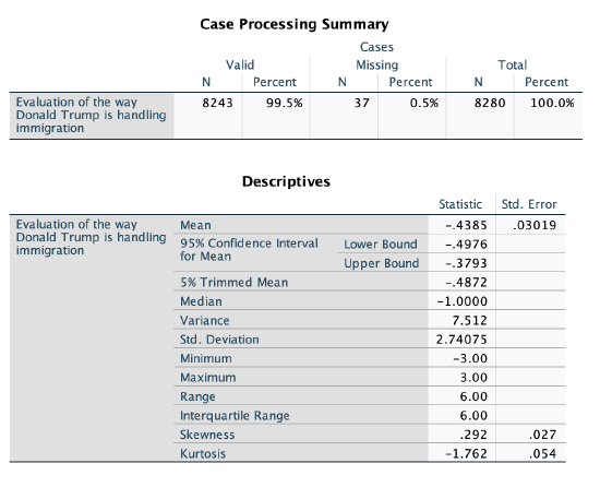
Respondents were asked, "Do you approve or disapprove of the way Donald Trump is handling immigration?" with the options "approve" or "disapprove." Respondents were then asked, "Do you [approve/disapprove] strongly or not strongly?"
I combined these into a new variable, coded from -3 to 3, where -3 is someone who strongly disapproves, -2 someone who disapproves but did not know or refused to answer the follow-up, -1 is someone who disapproves, but not strongly, 0 is someone who volunteered "don't know" to the first question, 1 is someone who approves, but not strongly, 2 is someone who approves but did not know or refused to answer the follow-up, and 3 is someone who strongly approves.
Independent Variables
Policy Position on Immigration
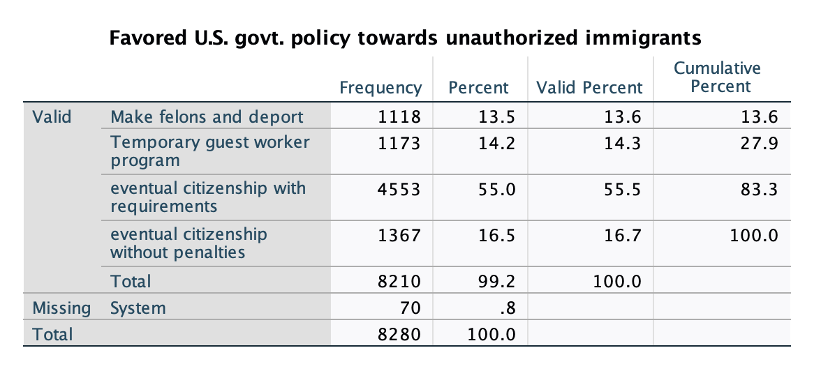
For the independent variables, views on immigration was captured by the question, "Which comes closest to your view about what government policy should be toward unauthorized immigrants now living in the United States?"
Potential responses (with re-coding) were:
0. Make all unauthorized immigrants felons and send them back to their home country
1. Have a guest worker program that allows unauthorized immigrants to remain in US to work but only for limited time
2. Allow unauthorized immigrants to remain in US & eventually qualify for citizenship but only if they meet requirements
3. Allow unauthorized immigrants to remain in US & eventually qualify for citizenship without penalties
This is an ordinal variable with only four categories, but I tested and it had a pretty linear relationship with the dependent variable, so I felt comfortable using it as ratio-like rather than making it into a reference group set.
Feelings towards Trump
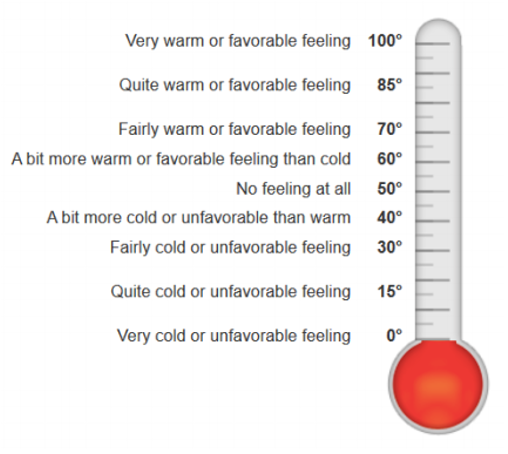
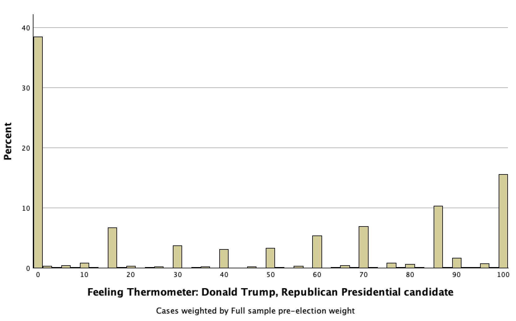
For feelings towards Trump, I used ANES' feelings thermometer question:
"I’d like to get your feelings toward some of our political leaders and other people who are in the news these days. I’ll read the name of a person and I’d like you to rate that person using something we call the feeling thermometer.
Ratings between 50 degrees and 100 degrees mean that you feel favorable and warm toward the person. Ratings between 0 degrees and 50 degrees mean that you don’t feel favorable toward the person and that you don’t care too much for that person. You would rate the person at the 50 degree mark if you don’t feel particularly warm or cold toward the person.
If we come to a person whose name you don’t recognize, you don’t need to rate that person. Just tell me and we’ll move on to the next one.
How would you rate: Donald Trump."
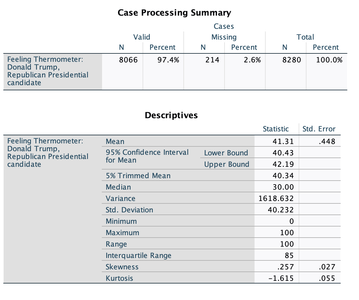
Bivariate Regressions
Let's start with two bivariate regressions. We've already covered these, so I'm just going to skip the SPSS parts and give you the summary display tables and graphs.
Policy Position on Immigration
Here's the first one:

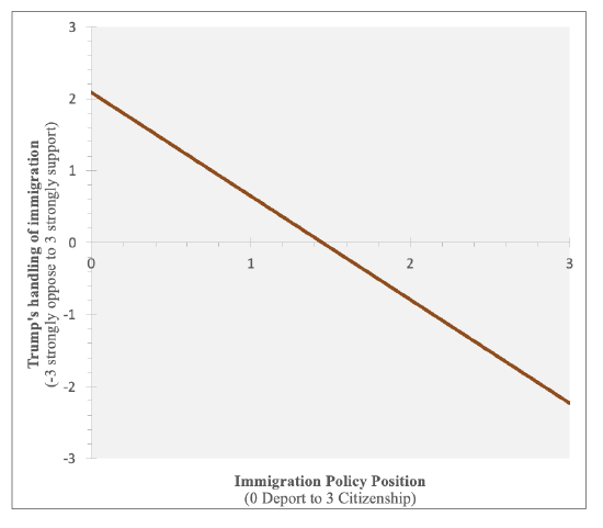
With a correlation of -0.47, there is a moderate negative relationship, with more liberal immigration views associated with less support for Trump's handling of immigration. Those who support unauthorized immigrants being felons and deported were predicted to support Trump's handling of immigration, while those who supported a path to citizenship without penalties were predicted to oppose Trump's handling of immigration. Views on immigration explain over 1/5 of variance in views on how Trump was handling immigration.
Feelings Towards Trump
Here's the second one:

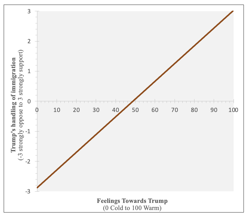
With a correlation of 0.87, there is a strong positive relationship, with warmer feelings towards Trump associated with more support for Trump's handling of immigration. Those with very cold feelings towards Trump are predicted to strongly oppose his handling of immigration and those with very warm feelings towards Trump are predicted to strongly support his handling of immigration. Respondents with a smidgeon colder than neutral feelings towards Trump (48.7 degrees) would be predicted to have neutral feelings on Trump's handling of immigration. Feelings towards Trump explain a whopping 3/4 of variance in views on how Trump was handling immigration.
Now let's combine them and do a multivariate regression.
Running Multivariate Regression with SPSS
Running multivariate linear regression in SPSS is an identical process to what we did in Chapter 13 when we had a reference group set. All the independent variables are put in simultaneously, either into the “Independent(s)” box if you are using drop-down menus or on the /METHOD=ENTER row if you are using syntax.
SPSS Outputs and Interpretations
Here is the output for my multivariate regression, using the two IVs from above, with some explanations and commentary:
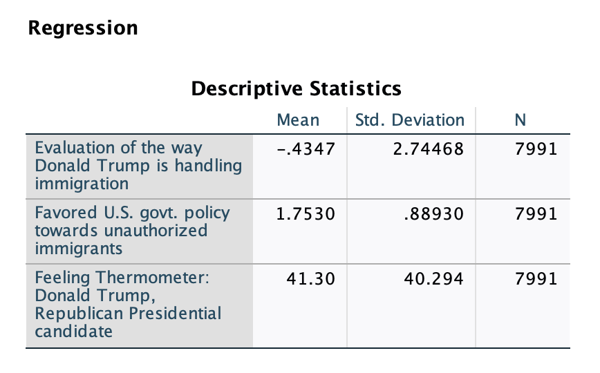
There is a smaller sample size than in the bivariate regressions, because we are only including cases that have valid data for all three variables.
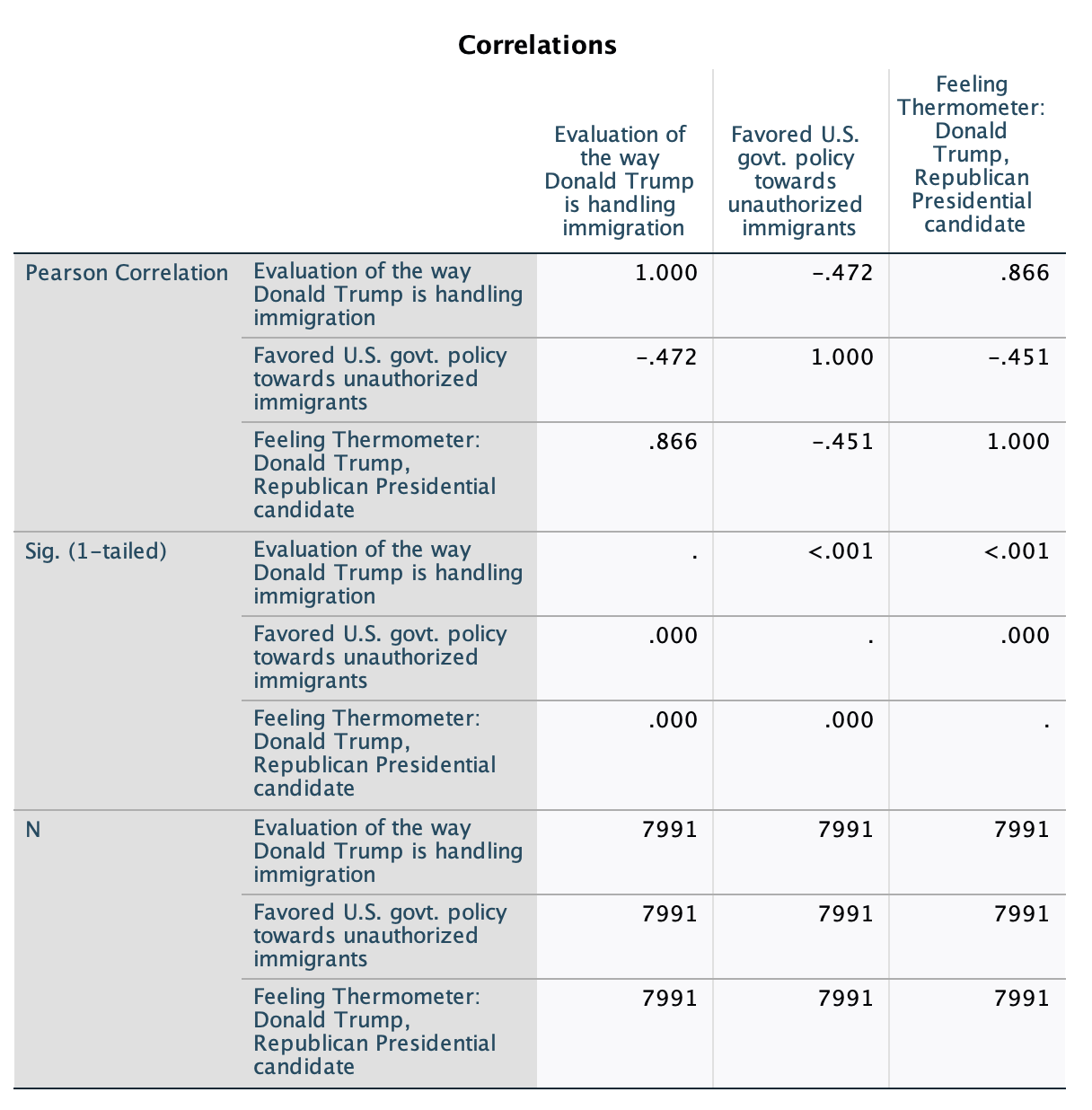
This output is a correlation matrix. Note that we can see individual Pearson's r correlation coefficient values for bivariate relationships. These also tell us whether these bivariate relationships are negative or positive. You can see that one of the IVs has a negative relationship with our DV and one has a positive relationship. This is why the model summary below only reports the overall strength of the model and not its direction.

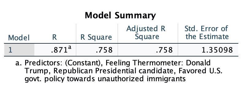
R-squared, explained variation, for the overall model
The model summary is based on including all of our independent variables. It does not tell us anything about either of them in isolation. This is the strength and explained variation for the overall model, accounting for both views on immigration policy and feelings towards Trump. Notice as well that you can't just add the (absolute value of the) r-values or r-squared values from the bivariate regressions together to get the overall model summary r-value and r-squared value. Our r-values from the bivariate regressions were -0.468 and 0.0866, which add up to a strength more than 1. Our r-squared values were 21.9% and 75.0%, which add up to 96.9%. Consider this: we can see in the bivariate correlation matrix above that our two independent variables have a moderate negative relationship. So there is overlapping explained variation. Once we already know feelings towards Trump, knowing immigration policy views does not improve our predictions by 21.9%, because some of that is already explained by feelings towards Trump. Similarly, if we already know immigration policy views, some of the 3/4 of explained variance from knowing feelings towards Trump was already accounted for, so we won't see a 75.0% boost on top of the 21.9% r-squared.
Interpretation of r: There is a strong relationship between our set of independent variables, views on immigration policy and feelings towards Trump, and support for Trump's handling of immigration.
Interpretation of r-squared: Views on immigration policy and feelings towards Trump together/collectively explain 75.8% of variance in support for Trump's handling of immigration (among respondents).
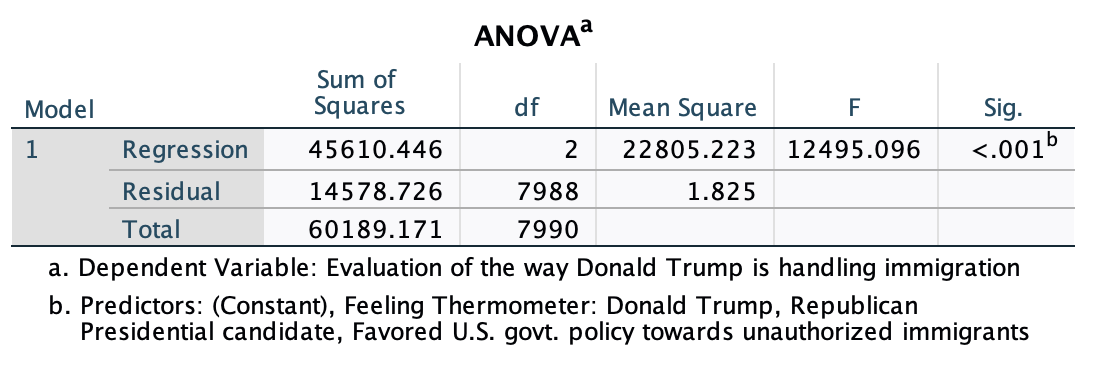
Overall Significance
For linear regression with one ratio-like or one indicator independent variable, our p-value from the ANOVA output was identical or near identical to the p-value for the slope of our independent variable. Now these may be different, because the p-value here is based on the full model: whether knowing all of our independent variables collectively improves our ability to predict the dependent variable over just knowing the mean of the dependent variable. This can be translated into a confidence level of whether r-squared is greater than zero. However, you could have one independent variable that helps and has a relationship and others that do not, and you could still have an ANOVA output with a p-value less than 0.05. This does not tell you about individual variables; rather, it is about the multivariate model as a whole.
The p-value is based on an F-test which is then converted into a p-value based on the F-distribution (which varies based on number of variables and sample size). Here is the formula that SPSS is using to calculate the F-statistic, where k is for the number of variables and n is for the sample size:
Interpretation: I am over 99.9% confident that there was a relationship between my independent variables, immigration policy views and feelings towards Trump, and my dependent variable, support for how Trump was handling immigration, among U.S. eligible voters leading up to the 2020 election.
This does not mean that each individual independent variable was actually helpful / was statistically significant in helping explain variation in support for how Trump was handling immigration. The ANOVA output box just speaks to the overall model. Technically p<0.001 means there is less than a 0.1% probability that we would have this data from a representative sample of our target population if, among our target population, knowing the collection of independent variables we put into the model does not improve our prediction of our DV over just knowing the mean of our DV.
If I did not know immigration policy views or feelings towards Trump, I would predict that a respondent would be at a -0.43 in their support for the way Trump is handling immigration, slightly unsupportive (this was the sample mean for the dependent variable). I am over 99.9% confident that, leading up to the 2020 election, for U.S. eligible voters, knowing immigration policy views and feelings towards Trump improves my prediction of support for the way Trump is handling immigration over just knowing the mean of support for the way Trump is handling immigration.

Slopes and Significance of Individual Independent Variables (and y-intercept), Part One
Remember with a reference group set how the constant, or y-intercept, was the value when all the indicator variables were zero? With a reference group set that was the reference group. Here, however, the y-intercept is the value when all the independent variables are zero. Therefore, now the y-intercept represents the point on the best fit line for a respondent who is both a 0 on immigration policy (favors deportation) and a 0 for feelings towards Trump (very cold).
We'll go over interpreting slopes below, but again note that the slopes here are different than in the bivariate regressions. It would be inaccurate to say that, for every one unit increase in support for more liberal immigration policies, support for the way Trump is handling immigration decreases by 0.3 units. As we know from the bivariate regression, for every one unit increase in support for more liberal immigration policies, support for the way Trump is handling immigration decreases by 1.4 units.
Therefore, whenever discussing individual variables from a multivariate model, we always add in language that notes this is while accounting for the other variable.
At the end of your explanation of the slope, or of the p-value, include language such as:
- "while controlling for [other independent variable name]" or
- "while holding [other independent variable name] constant."
These slopes are telling us the average impact in the sample for these independent variables while taking into consideration the other independent variable simultaneously. For example, the slope for immigration policy views indicates that, if you were to consider someone who feels cold towards Trump, or feels neutral, or feels warm, that among those people with the same feelings, we would predict an average of a 0.315 unit decrease in support for Trump's handling of immigration for every 1 unit increase in support for immigration policy views. The p-value is telling us whether we can be confident that, among our target population, the independent variable still has a relationship with the dependent variable after controlling for the other independent variable. Once we know (control for) feelings towards Trump, do immigration policy views still matter? If we take people who have the same feelings towards Trump (e.g., both somewhat cold, or both very warm, so holding this variable constant), is there a relationship, among those with the same feelings towards Trump, between immigration policy views and evaluation of the way Trump is handling immigration?
Unweighted:
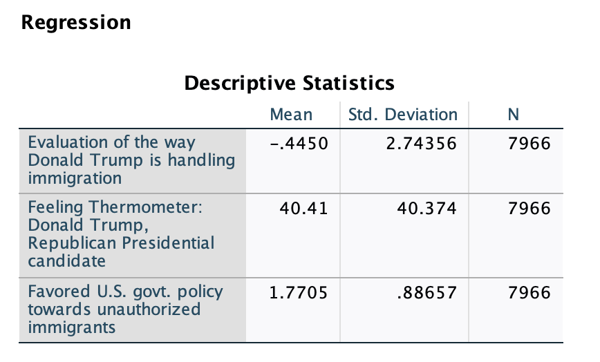
Just like before, I re-ran the regression without weighting to get the actual number of respondents.
Summary Display Table
I'm going to take the most useful information from above and put it into a summary display table.
Here is a Microsoft Word template for doing this. Fill out the red parts using the information from your SPSS output. MultivariateRegressionDisplayTableTemplate.docx
Here is what I filled out for the multivariate regression above. You should be able to find all the values and figure out the markers I used based on the outputs above.
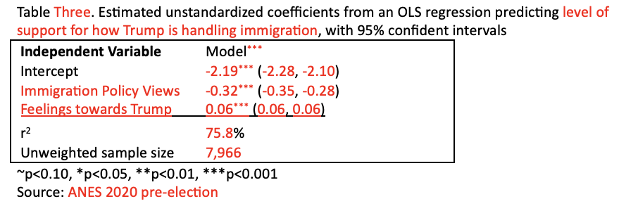
Here is a clean version without any parts in red:

Multivariate Linear Regression: Equation, Predictions, & Graphing
Before returning to our slopes, let's graph the regression, which will also help you visualize the relationships.
Linear Regression Equation
We will write out our one regression line equation the same way we did for reference group sets in Chapter 13: y=a+b1x1+b2x2 (and so forth depending on how many independent variables we have). Again, only make one regression equation, and include all your variables in it. You cannot make regression equations using only some of your independent variables without running a new regression that only includes those variables.
Here, instead of x1 I'm going to use P for policy views and instead of x2 I'm going to use F for feelings towards Trump.
y=a+bPP+bFF
y=(-2.19)+(-0.32)(P)+0.06(F)
To find any predicted dependent values for a given policy position and feelings thermometer degrees, plug in the values for P and F and solve for y.
For example, someone who supports eventual citizenship for unauthorized immigrants who meet certain requirements (P=2) and has fairly cold feelings towards Trump (F=30) would be predicted to disapprove, but not strongly, of Trump's handling of immigration (y=-1):
y=(-2.19)+(-0.32)(P)+0.06(F)
y=(-2.19)+(-0.32)(2)+0.06(30)
y=(-2.19)+(-0.64)+1.8
y=(-1.03)
Here is a template you can use if you would prefer to just put in your coefficients (y-intercept and slopes) and let Excel do the calculations for you: PredictedValueCalculator.MultivariateLinearRegression.xlsx
Who would be predicted to have the lowest dependent variable value, to oppose Trump's handling of immigration the most?
To get to the lowest y-value, our value for Policy views would need to be as high as possible, since its slope is negative, and our value for Feelings towards Trump would need to be as low as possible, since its slope is positive. Policy views goes from 0 to 3, so P=3, and Feelings towars Trump goes from 0 to 100, so F=0.
y=(-2.19)+(-0.32)(P)+0.06(F)
y=(-2.19)+(-0.32)(3)+0.06(0)
y=(-3.15)
Someone who supports unauthorized immigrants eventually qualifying for citizenship without penalties (P=3) and has very cold feelings towards Trump (F=0) would be predicted to strongly oppose Trump's handling of immigration (beyond the lower bound of -3).
Who would be predicted to have the highest dependent variable value, to support Trump's handling the most?
To get to the highest y-value, our Policy views value would need to be as low as possible, since its slope is negative, and our Feelings thermometer value would need to be as high as possible, since its slope is positive. P goes from 0 to 3, so P=0, and F goes from 0 to 100, so F=100.
y=(-2.19)+(-0.32)(P)+0.06(F)
y=(-2.19)+(-0.32)(0)+0.06(100)
y=(3.81)
Someone who supports making unauthorized immigrants felons and deporting them (P=0) and has very warm feelings towards Trump (F=100) would be predicted to strongly support Trump's handling of immigration (beyond the upper bound of +3).
Graphing
Here is a template for making multivariate linear regression graphs: MutlvariateLinearRegressionGraphTemplate.xlsx
Our graphs will only be of two independent variables (if using a reference group set, that can count as one variable). If you have three or more variables, you need to hold the other variables constant (e.g., you would use two independent variables, such as age and income, and then hold other variables at a value you select, such as race=white, marital status=married, gender=woman, etc.) You can then replace the variables in your equation with those constant values to simplify your equation and graph it. The graph will show the relationship accounting for the two independent variables, while holding the others constant (e.g. a graph of the predicted relationship between age and income with the dependent variable, among white married women).
If you have two categorical variables (e.g., two indicator variables, two reference group sets, one indicator variable and one reference group set), you will need to make a bar graph. (If you have more than two IVs, you only need to make a bar graph if the two IVs you want to show in terms of relationships are both categorical.) Here is an example of a bar graph where the IVs were gender (indicator) and marital status (reference group set):
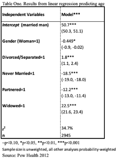
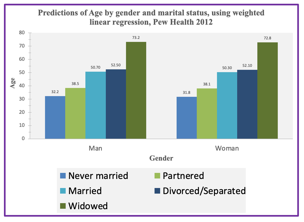
However, if at least one of your variables is ratio-like, you can make a line graph.
If only one of your independent variables is ratio-like, that is the variable that will go on the x-axis. If they are both ratio-like, you can choose which variable goes on the x-axis. In general, if you have a variable that has more of a spread (e.g., age from 18 to 89, feelings thermometer temperatures from 0 to 100, income, etc.), those are better variables to go on the x-axis than ones that are ratio-like but have fewer categories or ones that are ratio-level but still have only a few categories (e.g., number of siblings, age if everyone is 10, 11, or 12 years old, a Likert scale variable that goes from -2 to +2, etc.).
The independent variable that is not going on the x-axis will be presented by different lines. You need to choose a few different values to show for this variable. You will be holding this variable constant at these various values. For example, for a feelings thermometer variable, I might choose 0, 50, and 100. For a strongly agree to strongly disagree variable I might choose strongly agree, strongly disagree, and neutral. If there are not many respondents at these extremes, I might choose values closer to the center, e.g., for the feelings thermometer: 30 (fairly cold), 50 (neutral), and 70 (fairly warm); for a Likert Scale: agree and disagree rather than strongly agree and strongly disagree.
For this multivariate regression, I will put the feelings thermometer on the x-axis, since it goes from 0 to 100, whereas policy views only has 4 options. Because there are only 4 options for the policy views variable, I am going to graph all 4 of them rather than just choosing 2 or 3. For my graph, each line will represent a different policy view.
Here is the first part of the template for a four-line graph:
Here are the coefficients I need:
Here is what I put into the top part of the template:
My independent variable for the x-axis, the feelings thermometer, goes from 0 to 100, with cases at its minimum and maximum.
My independent variable I am holding constant for the four lines, the policy views variable, goes from 0 to 3, with cases at its minimum and maximum.
Here is what I put in for the next part of the template:
Finally, I edited my axes labels and my x-axis and y-axis bounds and units. For the x-axis, I'm using the feelings thermometer variable, so I made the bounds 0 to 100, major units 10, and minor units 2. Here is what my final graph looks like:
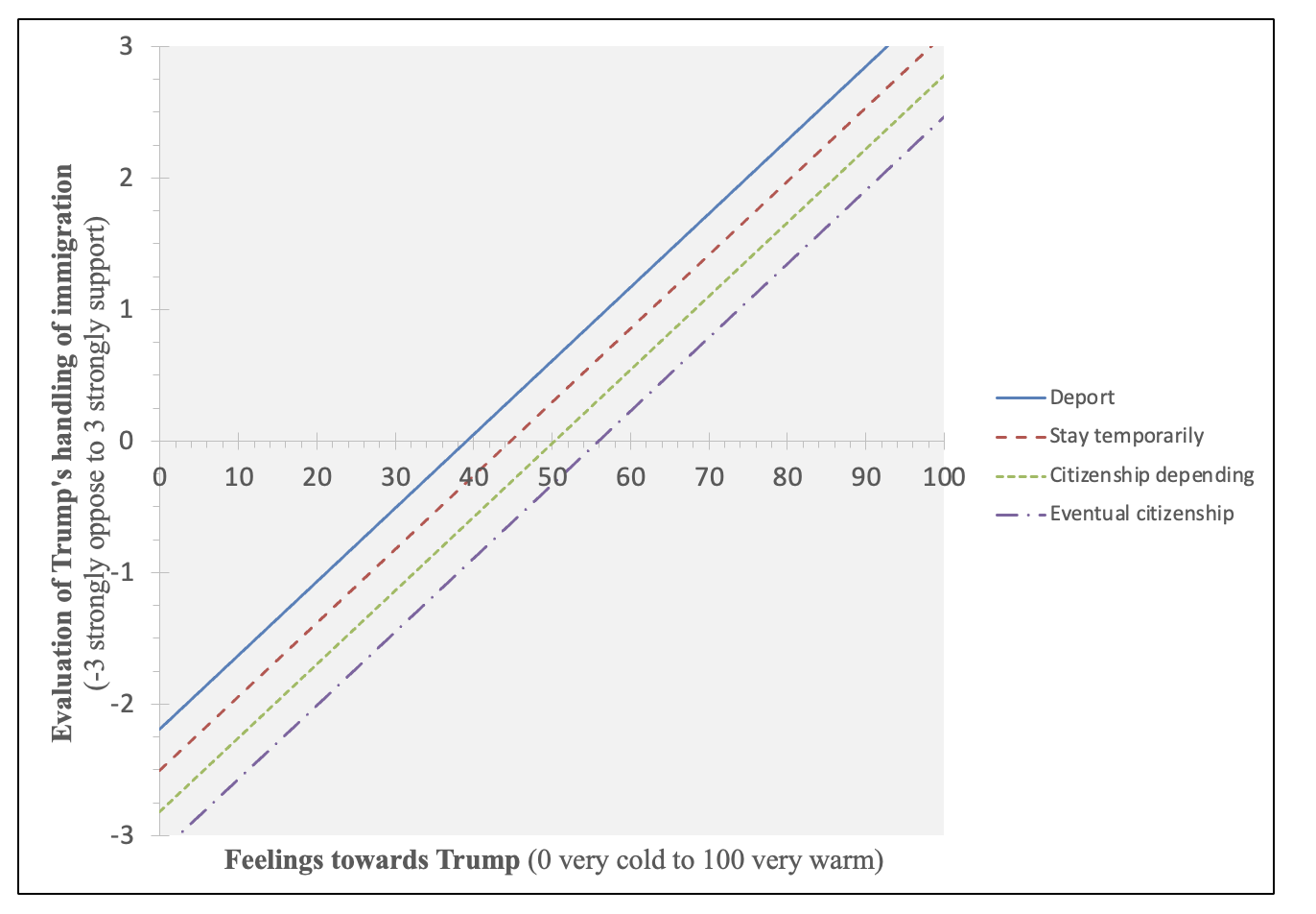
You can see that, across policy positions, as feelings towards Trump get warmer, support for Trump's handling of immigration increases. Also, you can see that at any given feeling towards Trump, people with more liberal policy positions are less supportive of Trump's handling of immigration and people with more conservative policy positions are more supportive of Trump's handling of immigration.
Slopes and Significance of Individual Independent Variables (and y-intercept), Continued (Part Two)
Let's return to the y-intercept, slopes, and their p-values, and interpret them in context.
Y-intercept: -2.189, p-<0.001
The y-intercept is the predicted value when all IVs are zero. y=(-2.19)+(-0.32)(0)+0.06(0)=(-2.19)
In this case, this is someone at a 0 (very cold) in their feelings towards Trump and a 0 (deport) in their policy position on immigration.
In the line graph above, find the solid blue line and where it intersects with the y-axis (where the x-axis value is 0). You can see that it is at -2.19.
We would predict that someone who feels very cold towards Trump and supports deporting unauthorized immigrants would be at a -2.2, supportive of Trump's handling on immigration.
The p-value means we are over 99.9% confident that, among our target population, the y-intercept is not zero. In this case, that means that we are over 99.9% confident that, among U.S. eligible voters leading up to the 2020 election, someone who feels very cold towards Trump and supports deporting unauthorized immigrants would not be predicted to be neutral (at a 0) in their evaluation of Trump's handling of immigration.
Slopes (template):
Interpreting each slope is the same as what we did in bivariate linear regression, except this time you need to add "while holding [the other IV(s) constant]" or "while controlling for [the other IVs]".
P-values (template):
Interpreting each p-value is the same as what we did in bivariate linear regression, except this time you need to add "while holding [the other IV(s) constant]" or "while controlling for [the other IVs]".
Contextualize these by naming the other IV(s).
(If you had a lot of independent variables, you would not name all the other variables.)
Immigration policy views: -0.32, p<0.001
- The slope for immigration policy views, while holding feelings towards Trump constant, is -0.32.
- That means that, while controlling for feelings towards Trump, for every one-unit increase in immigration policy views, support for Trump's immigration handling goes down by 0.32.
- Look up at the graph. Hold feelings towards Trump constant by choosing any feelings thermometer temperature and drawing an imaginary vertical line on the graph. For example, take a look at when feelings towards Trump are at 70, fairly warm. Because this variable is coded in one-unit increments and I graphed lines for every value, you can literally see the slope as you move from line to line. Each unit increase for the independent variable, which goes from 0 to 1, and then 1 to 2, and then 2 to 3, represents the change: from deport to stay temporarily, from stay temporarily to eventual citizenship with conditions, from eventual citizenship with conditions to eventual citizenship without penalties. As you go straight down at any given feelings thermometer temperature, you will see that as policy views goes from 0 to 3, it goes down by 0.32 points each time. On average, every one unit increase in immigration policy views (becoming more liberal, from 0 at deport to 3 at eventual citizenship without penalties) is associated with a respondent's support for Trump's handling of immigration decreasing by an average of 0.32 (from -3 strongly oppose to +3 strongly support), while controlling for feelings towards Trump.
- The p-value means we are over 99.9% confident that, among our target population, the slope is not zero, when controlling for the other independent variable(s). In this case, that means we are over 99.9% confident that, among U.S. eligible voters leading up to the 2020 election, there is a relationship between policy positions on immigration and support for how Trump is handling immigration, while holding feelings towards Trump constant.
Feelings towards Trump: 0.06, p<0.001
- The slope for feelings towards Trump, while holding policy positions on immigration constant, is 0.06.
- That means that, while controlling for policy positions on immigration, for every one degree warmer a respondent's feelings towards Trump are, support for Trump's immigration. handling goes up by 0.06.
- Look up at the graph. Hold policy positions constant by choosing any one line to follow. They all have the same slope of 0.06. As you go across from left to right, every one degree warmer (in feelings towards Trump) goes up by 0.06 (1% of the distance of the -3 to +3 scale). Every 10 degrees warmer goes up by 0.6. For an increase of 50 degrees warmth (e.g., from 0 to 50, or 50 to 100, or 20 to 70, etc.), the dependent variable goes up by 3 units, half the scale of -3 to +3. You can see how much support for Trump's immigration handling goes up as feelings get warmer towards Trump, while controlling for policy positions on immigration.
- The p-value means we are over 99.9% confident that, among our target population, the slope is not zero, when controlling for the other independent variable(s). In this case, that means we are over 99.9% confident that, among U.S. eligible voters leading up to the 2020 election, there is a relationship between feelings towards Trump and support for how Trump is handling immigration, while holding policy positions on immigration constant.
Beta (standardized) Slopes: Comparing IV Contributions
In the multivariate model, which has a more substantive impact? Policy positions on immigration or feelings towards Trump?
At first glance, you might assume it's policy positions on immigration, as the slope is larger (-0.32 vs. 0.06). However, policy positions on immigration only has 6 one-unit increments on its 7-category scale, whereas feelings towards Trump can vary from 0 to 100. Furthermore, respondents are not equally distributed across these scales, and so if people have more uniform responses for one of the variables, it might not explain as much about the dependent variable. So, from what we've learned so far, it's difficult to tell.
The way we can make comparisons between slopes is by using a different type of slope, called a Beta or standardized slope.
Beta slopes, or standardized slopes, are slopes with standard deviations as their unit.
Beta or standardized slopes are slopes based on standard deviations. They make the unit for all independent variables' slopes into standard deviations.

Whereas for our unstandardized slopes, the units are whatever they are (e.g., degrees on the feelings thermometer or dollars for income), for standardized slopes, the units are all standard deviations.
- An unstandardized slope's interpretation is: Every one unit increase in x is associated with an increase in y of (unstandardized slope value) units.
- A standardized slope's interpretation is: Every one standard deviation increase in x is associated with an increase in y of (beta slope value) standard deviations.
You can find standardized slopes in your SPSS output.

They are in the "Standardized Coefficients, Beta" column of the coefficients output. Here the standardized slope for immigration policy position is -0.102 and the standardized slope for feelings towards Trump is 0.820.
Immigration Policy Views Slopes
Unstandardized: Every one unit increase in immigration policy views (becoming more liberal on the 0 to 3 scale) is associated with a 0.315 unit decrease in support for Trump's handling of immigration (on the -3 to 3 scale), while holding feelings towards Trump constant.
Standardized: Every one standard deviation increase in immigration policy views is associated with a decrease of 0.102 standard deviations in support for Trump's handling of immigration, while holding feelings towards Trump constant.
Feelings Towards Trump Slopes
Unstandardized: Every one degree warmer in feelings towards Trump (on the 0 to 100 scale) is associated with a 0.56 unit decrease in support for Trump's handling of immigration (on the -3 to 3 scale), while holding policy positions on immigration constant.
Standardized: Every one standard deviation increase in feelings towards Trump is associated with an increase of 0.820 standard deviations in support for Trump's handling of immigration, while holding policy positions on immigration constant.
Beta slopes are not very intuitive in terms of their interpretations.
What does it look like when policy positions on immigration increase by one standard deviation, or feelings towards Trump increases by one standard deviation, or evaluations of Trump's handling on immigration decreases by 0.1 or increases by 0.8 standard deviations?
I can use the standard deviations of each variables to translate these standard deviations back into the units that the original coding of the variable uses.

- A one standard deviation increase in policy positions on immigration is a 0.89 unit increase on the 0 to 3 scale.
- A one standard deviation increase in feelings towards Trump is 40 degrees warmer on the feelings thermometer.
- A decrease of 0.1 standard deviations in evaluations of Trump's handling of immigration is a 0.28 unit decrease on the -3 to +3 scale.
- An increase of 0.8 standard deviations in evaluations of Trump's handling of immigration is a 2.25 unit increase on the -3 to +3 scale.
So for example, for the Beta slope for feelings towards Trump:
Every one standard deviation increase (40 degrees warmer) in feelings towards Trump is associated with an increase of 0.820 standard deviations (a 2.25 unit decrease) in support for Trump's handling of immigration, while holding policy positions on immigration constant.
These are still not very helpful.
However, beta slopes are useful for comparing the contribution of each independent variable to the dependent variable. We can't tell this from unstandardized slopes, as we are often comparing apples to oranges (the variables may have different units, different variances, etc.).
When using beta slopes to compare which independent variable has more of an impact, just consider their absolute value (distance from zero). We don't care if the slope is positive or negative for considering its impact.
Here, 0.82 > 0.10, so feelings towards Trump has more of an impact than policy positions on immigration. It has about 8 times more impact. This is the opposite conclusion we would have come to if we had just evaluated the unstandardized coefficients.
Comparing Bivariate and Multivariate Regressions
Remember when we looked at elaborated/partial crosstabs in Chapter 9? We compared bivariate to multivariate relationships.
Here was a summary of what happened when we introduced a new control variable:
- The initial relationship stays the same
- Replication: relationship still exists
- The initial relationship goes away
- If control variable is antecedent
- Spurious: Relationship explained by control (confounding) variable
- If control variable is intervening
- Relationship's mechanism explained by control (mediating) variable
- If control variable is antecedent
- The initial relationship diminishes
- If control variable is antecedent
- Relationship is partially explained by control variable, but original independent variable still has its own independent effect
- If control variable is intervening
- Relationship's mechanism is partially but not fully explained by control variable
- If control variable is antecedent
- The initial relationship varies
- Moderation: relationship differs/interacts with control variable
- The initial relationship increases (or there was no relationship, and now a relationship appears)
- Suppression: Relationship was suppressed, relationship is explained by its effect within control variable groups
Similar to when we added a second independent variable into a crosstab, we can analyze what happens when we introduce an additional independent variable or variables into our bivariate model using linear regression.
For example, I could ask: do people evaluate Trump's handling of immigration policy based on their own views on immigration (in comparison to what Trump is doing), or do their feelings about Trump trump their views on immigration? Once I already know people's policy positions on immigration, does knowing their feelings towards Trump improve our predictions further? (Or vice versa, does feelings towards Trump improve our prediction of people's evaluations of Trump's handling of immigration? And once we know how people feel overall about Trump, does knowing their policy positions on immigration improve our predictions of Trump's handling of immigration further?)
We can compare our two bivariate regressions and our multivariate regression altogether in one summary display table. We want to pay attention to what happens to the r-squared, significance of the independent variables, and slopes when we move from the bivariate to multivariate regressions.
Here is a template for doing this: LinearRegression.MultipleModels.DisplayTableTemplate.xlsx
Each column is a model/regression. For the bivariate models, you leave blank the variable that is not part of your regression. The final column is called the "full model" because it contains all of your independent variables.
- Don't forget to update the *** which are already listed as asterisks rather than question marks in this template.
- Note that in Excel, you cannot start a cell by typing a - sign or it will think it's a formula. To correct this, type ' before the - sign. For example, to write -3.5* you would input '-3.5*. This tells Excel it is just text.
Since I have two ratio-like variables, I'm using the first template worksheet, which looks like this:
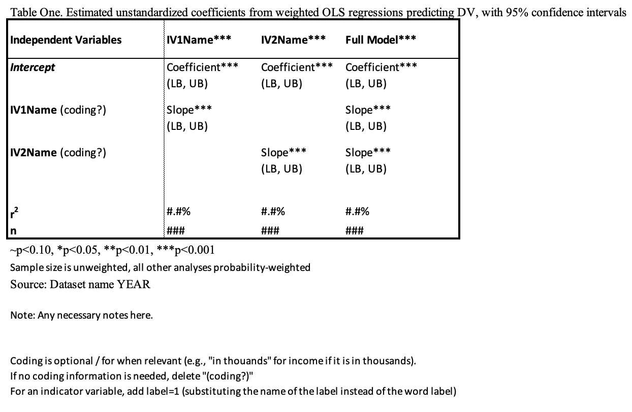
I'm just taking the information from the summary display tables earlier in this chapter (Tables One, Two, and Three) and putting them each into one of the columns:

Now I can make comparisons between the bivariate and multivariate model. Both independent variables are significant in both the bivariate and multivariate regressions. This means that both are having an effect on how U.S. eligible voters prior to the 2020 election were evaluating Trump's handling of immigration, while controlling for the other (both improve our prediction, even after we know the other).
The r-squared of the full model is less than 1% greater than the r-squared of feelings towards Trump model, but over 50% more than the immigration policy views model. This means that among our respondents, if you already know immigration policy views, knowing feelings towards Trump will substantially improve the explained variation of evaluations of Trump's handling on immigration, but if you already know feelings towards Trump, also knowing immigration views will not add much explanatory power.
Finally, let's take a look at slopes. The feelings thermometer for Trump slope stays identical (when rounded to the nearest hundredths place) after controlling for immigration policy views. It is unaffected by policy views on immigration. However, we can see that the slope for immigration policy views drops from -1.44 to -0.32. The initial slope was 4.5 times larger than the slope after controlling for feelings thermometer. This means that feelings towards Trump partially explains the relationship between immigration policy views and evaluations of Trump's handling on immigration. Depending on which independent variable comes first time-order wise, this could mean that for many but not all respondents, their feelings on Trump are impacting their views on immigration based on them taking cues from Trump (or distancing themselves from Trump) for their views on immigration, or it could mean that many respondent's positions on immigration are impacting their feelings towards Trump and their evaluation of Trump's handling on immigration in a similar direction, or it could be some combination of these two. Based on the confidence intervals for the slopes, we can be confident about these claims for U.S. eligible voters leading up to the 2020 election as a whole, not just our respondents.
What is the overall story here? Originally when we looked at immigration policy views, we saw that it had a substantive impact on evaluating Trump's handling of immigration. But this is not the whole story. It's not only immigration policy views that are impacting how people evaluate Trump's handling of immigration. Once we controlled for feelings towards Trump, we saw this relationship diminish substantially, indicating that it is partially explained by feelings towards Trump. Additionally, we saw that feelings towards Trump by itself (the bivariate model) explains 3/4 of variation in evaluation of Trump's handling on immigration --- ignoring people's policy positions on immigration, which by itself explained about 1/5 of the variation in evaluation of Trump's handling on immigration. People's evaluations of Trump's handling on immigration is influenced more by feelings towards Trump than by policy positions on immigration. While there are some people whose policy positions on immigration are influencing their evaluation of Trump's handling on immigration, people's evaluation of Trump's handling of immigration are most influenced by how people overall feel about Trump, not by whether their policy positions on immigration align with Trump's handling of immigration.


