
6: Comparing Confidence Intervals
- Page ID
- 188425

\( \newcommand{\vecs}[1]{\overset { \scriptstyle \rightharpoonup} {\mathbf{#1}} } \)
\( \newcommand{\vecd}[1]{\overset{-\!-\!\rightharpoonup}{\vphantom{a}\smash {#1}}} \)
\( \newcommand{\dsum}{\displaystyle\sum\limits} \)
\( \newcommand{\dint}{\displaystyle\int\limits} \)
\( \newcommand{\dlim}{\displaystyle\lim\limits} \)
\( \newcommand{\id}{\mathrm{id}}\) \( \newcommand{\Span}{\mathrm{span}}\)
( \newcommand{\kernel}{\mathrm{null}\,}\) \( \newcommand{\range}{\mathrm{range}\,}\)
\( \newcommand{\RealPart}{\mathrm{Re}}\) \( \newcommand{\ImaginaryPart}{\mathrm{Im}}\)
\( \newcommand{\Argument}{\mathrm{Arg}}\) \( \newcommand{\norm}[1]{\| #1 \|}\)
\( \newcommand{\inner}[2]{\langle #1, #2 \rangle}\)
\( \newcommand{\Span}{\mathrm{span}}\)
\( \newcommand{\id}{\mathrm{id}}\)
\( \newcommand{\Span}{\mathrm{span}}\)
\( \newcommand{\kernel}{\mathrm{null}\,}\)
\( \newcommand{\range}{\mathrm{range}\,}\)
\( \newcommand{\RealPart}{\mathrm{Re}}\)
\( \newcommand{\ImaginaryPart}{\mathrm{Im}}\)
\( \newcommand{\Argument}{\mathrm{Arg}}\)
\( \newcommand{\norm}[1]{\| #1 \|}\)
\( \newcommand{\inner}[2]{\langle #1, #2 \rangle}\)
\( \newcommand{\Span}{\mathrm{span}}\) \( \newcommand{\AA}{\unicode[.8,0]{x212B}}\)
\( \newcommand{\vectorA}[1]{\vec{#1}} % arrow\)
\( \newcommand{\vectorAt}[1]{\vec{\text{#1}}} % arrow\)
\( \newcommand{\vectorB}[1]{\overset { \scriptstyle \rightharpoonup} {\mathbf{#1}} } \)
\( \newcommand{\vectorC}[1]{\textbf{#1}} \)
\( \newcommand{\vectorD}[1]{\overrightarrow{#1}} \)
\( \newcommand{\vectorDt}[1]{\overrightarrow{\text{#1}}} \)
\( \newcommand{\vectE}[1]{\overset{-\!-\!\rightharpoonup}{\vphantom{a}\smash{\mathbf {#1}}}} \)
\( \newcommand{\vecs}[1]{\overset { \scriptstyle \rightharpoonup} {\mathbf{#1}} } \)
\(\newcommand{\longvect}{\overrightarrow}\)
\( \newcommand{\vecd}[1]{\overset{-\!-\!\rightharpoonup}{\vphantom{a}\smash {#1}}} \)
\(\newcommand{\avec}{\mathbf a}\) \(\newcommand{\bvec}{\mathbf b}\) \(\newcommand{\cvec}{\mathbf c}\) \(\newcommand{\dvec}{\mathbf d}\) \(\newcommand{\dtil}{\widetilde{\mathbf d}}\) \(\newcommand{\evec}{\mathbf e}\) \(\newcommand{\fvec}{\mathbf f}\) \(\newcommand{\nvec}{\mathbf n}\) \(\newcommand{\pvec}{\mathbf p}\) \(\newcommand{\qvec}{\mathbf q}\) \(\newcommand{\svec}{\mathbf s}\) \(\newcommand{\tvec}{\mathbf t}\) \(\newcommand{\uvec}{\mathbf u}\) \(\newcommand{\vvec}{\mathbf v}\) \(\newcommand{\wvec}{\mathbf w}\) \(\newcommand{\xvec}{\mathbf x}\) \(\newcommand{\yvec}{\mathbf y}\) \(\newcommand{\zvec}{\mathbf z}\) \(\newcommand{\rvec}{\mathbf r}\) \(\newcommand{\mvec}{\mathbf m}\) \(\newcommand{\zerovec}{\mathbf 0}\) \(\newcommand{\onevec}{\mathbf 1}\) \(\newcommand{\real}{\mathbb R}\) \(\newcommand{\twovec}[2]{\left[\begin{array}{r}#1 \\ #2 \end{array}\right]}\) \(\newcommand{\ctwovec}[2]{\left[\begin{array}{c}#1 \\ #2 \end{array}\right]}\) \(\newcommand{\threevec}[3]{\left[\begin{array}{r}#1 \\ #2 \\ #3 \end{array}\right]}\) \(\newcommand{\cthreevec}[3]{\left[\begin{array}{c}#1 \\ #2 \\ #3 \end{array}\right]}\) \(\newcommand{\fourvec}[4]{\left[\begin{array}{r}#1 \\ #2 \\ #3 \\ #4 \end{array}\right]}\) \(\newcommand{\cfourvec}[4]{\left[\begin{array}{c}#1 \\ #2 \\ #3 \\ #4 \end{array}\right]}\) \(\newcommand{\fivevec}[5]{\left[\begin{array}{r}#1 \\ #2 \\ #3 \\ #4 \\ #5 \\ \end{array}\right]}\) \(\newcommand{\cfivevec}[5]{\left[\begin{array}{c}#1 \\ #2 \\ #3 \\ #4 \\ #5 \\ \end{array}\right]}\) \(\newcommand{\mattwo}[4]{\left[\begin{array}{rr}#1 \amp #2 \\ #3 \amp #4 \\ \end{array}\right]}\) \(\newcommand{\laspan}[1]{\text{Span}\{#1\}}\) \(\newcommand{\bcal}{\cal B}\) \(\newcommand{\ccal}{\cal C}\) \(\newcommand{\scal}{\cal S}\) \(\newcommand{\wcal}{\cal W}\) \(\newcommand{\ecal}{\cal E}\) \(\newcommand{\coords}[2]{\left\{#1\right\}_{#2}}\) \(\newcommand{\gray}[1]{\color{gray}{#1}}\) \(\newcommand{\lgray}[1]{\color{lightgray}{#1}}\) \(\newcommand{\rank}{\operatorname{rank}}\) \(\newcommand{\row}{\text{Row}}\) \(\newcommand{\col}{\text{Col}}\) \(\renewcommand{\row}{\text{Row}}\) \(\newcommand{\nul}{\text{Nul}}\) \(\newcommand{\var}{\text{Var}}\) \(\newcommand{\corr}{\text{corr}}\) \(\newcommand{\len}[1]{\left|#1\right|}\) \(\newcommand{\bbar}{\overline{\bvec}}\) \(\newcommand{\bhat}{\widehat{\bvec}}\) \(\newcommand{\bperp}{\bvec^\perp}\) \(\newcommand{\xhat}{\widehat{\xvec}}\) \(\newcommand{\vhat}{\widehat{\vvec}}\) \(\newcommand{\uhat}{\widehat{\uvec}}\) \(\newcommand{\what}{\widehat{\wvec}}\) \(\newcommand{\Sighat}{\widehat{\Sigma}}\) \(\newcommand{\lt}{<}\) \(\newcommand{\gt}{>}\) \(\newcommand{\amp}{&}\) \(\definecolor{fillinmathshade}{gray}{0.9}\)In Chapter 5 we explored confidence intervals and how we can make inferential claims about our target population based on representative sample data. In this chapter we'll again make inferential claims and explore confidence intervals, but this time we will compare confidence intervals, including among subgroups. When we have representative sample data, we can compare means and proportions at the population level. This chapter will also introduce language of significance and substantiveness, which will be followed up on in more depth in Chapter 7.
With our 24/7 news cycle, we are inundated with discussion of poll results, and small changes in polls often get blasted out as important and meaningful. Take this summer 2023 news release: "Reuters/Ipsos Survey: Despite indictments, Trump leads primary field as DeSantis loses support." The headline is supported by this claim: "Former President Donald Trump continues to lead the Republican primary field (47%). At the same time, Florida Governor Ron DeSantis’ support has dropped to 13%, a six-point drop from mid-July."
This poll uses a non-probability online sample, where respondents have been recruited into panels or click on online advertisements. While Reuters/Ipsos uses weighting, this cannot account for if the people in the sample are different from people who share their demographics that were not in the sample. Because it is not a probability sample, we would not do inferential statistics or build a confidence interval. Reuters/Ipsos, however, uses something called a "credibility interval." The American Association for Public Opinion Research states they are concerned with underlying biases associated with nonprobability online samples, though they also note traditional probability samples can also be problematic when they have areas of noncoverage and high levels of nonparticipation. For our purposes here, however, let's use the "credibility interval" as if it were a regular "margin of error" and look at the poll results and inferential statistics in kind.
Does Trump lead the primary field? Trump's sample proportion was 47%.
The confidence/credibility interval will be: 47% ± 6.4%, so among all Republicans, support for Trump was somewhere between 41.6% to 53.4%.
The next highest polling candidate, DeSantis, is at 13%. 13% ± 6.4% gives us a range of 6.6% to 19.4%.
The headline indicating that "Trump leads primary field" seems accurate.
The graph below shows the percentage each candidate got among the 365 Republican respondents in the sample, along with a line that represents the confidence interval for where we could reasonably expect the actual percentage of support to be among all U.S. Republicans.
We can see that, even taking into account the confidence intervals, Trump is leading the pack. If this were a traditional confidence interval, we would say that, at the 95% confidence level, the lowest support Trump might have is 41.6%, and the highest any other candidates might have is DeSantis at 19.4%. These confidence intervals do not touch or overlap, meaning that we are over 95% confident that, among all U.S. Republicans (at the time of the poll), there was more support for Trump than for DeSantis or other candidates. We refer to this as being "significantly" different.
If we are over 95% confident that two proportions (or means) are different, they are significantly different.
Statistical significance is a technical statistics term. It does not mean that the difference is meaningful or important, just that we are over 95% confident it exists among our target population. If two 95% confidence intervals do not overlap, the proportions/means are significantly different.
Is DeSantis ahead of Pence? DeSantis was 2nd place in the poll, at 13%, while Pence was 3rd place in the poll, at 8%. So 1/20 more Republican surveytakers preferred DeSantis to Pence. But again, we don't really care about the 365 Republicans who were surveyed. We want to know about all U.S. Republicans' preferences. If you look at the confidence intervals, they overlap.
If two 95% confidence intervals overlap, the proportions/means are not significantly different. They could be the same. At the 95% confidence level, DeSantis could be ahead of Pence, Pence could be ahead of DeSantis, or they could be tied. Thus, even though the sample proportions are different, the two are not significantly different. We cannot be over 95% confident that, among all U.S. Republicans, DeSantis is ahead of Pence or that DeSantis has a different level of support from Pence.
Sometimes you will see significance language in news stories. For example, check out the excerpts below from the article, "Poll finds dead heat in Mississippi governor's race." I bolded the language that refers to the concept of statistical significance. When the article says there is a statistical tie or an insignificant difference, it means that when accounting for sampling error, we cannot be over 95% confident that either candidate has the lead among our target population.
Two titans of Mississippi politics are statistically tied in the race for governor, a new survey shows, highlighting what will be one of the marquee matchups in what might otherwise be a quiet political year.
The survey, conducted by the nonpartisan firm Mason-Dixon Polling and Strategy, finds Attorney General Jim Hood (D) holding a slim two-point lead over Lt. Gov. Tate Reeves (R), 44 percent to 42 percent, a statistically insignificant edge in a poll with a margin of error of plus or minus 4 percentage points.
If retired Supreme Court Justice Bill Waller runs as an independent, Hood would cling to a similarly insignificant 40 percent to 38 percent lead over Reeves. Waller takes 9 percent of the vote in that scenario.
While we determined that Trump has a significant lead over his primary opponents, it does not mean the difference is sizable. If we were over 95% confident that Trump had 0.0001% more support among U.S. Republicans than other candidates, he would still have a significant lead. It's not the dictionary definition of significant.
This then leads us to our next question, whether or not the difference is substantive.
In the poll sample, Trump was 34% ahead of DeSantis, 47% to 13%. However, with our 95% confidence intervals, Trump could be anywhere from 22.2% to 46.8% ahead of DeSantis. We are 95% confident that Trump is at least 22.2% ahead of DeSantis among U.S. Republicans.
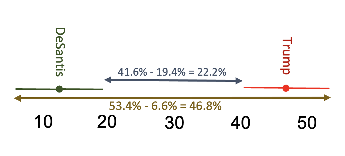
To figure those numbers out, I looked at how close together the confidence intervals could be. I subtracted the upper bound of DeSantis' confidence interval from the lower bound of Trump's confidence interval. I am 95% confident that they are at least that far apart. To find out at most how far apart they might be at the 95% confidence level, I subtracted the lower bound of DeSantis' confidence interval from the upper bound of Trump's confidence interval.
Given that I am 95% confident that at over 1 in 5 more Republicans prefer Trump to DeSantis, this is a substantive difference.
A difference that is big, sizable, notable. A difference we care about. If possible, we evaluate this at the population rather than sample level.
For comparing support between DeSantis and Pence, if we are not even confident a relationship exists, then it's not going to be substantive either. Unless we are making a Type 2 error (a false negative, claiming there is not a significant difference when actually there is a difference among all U.S. Republicans between support for DeSantis and Pence), insignificant relationships are not substantive.
Going back to the article's original claims, the next part of the headline was that DeSantis lost support, with a supporting claim that he had lost 6% support over the past month. On the surface, this seems to likely not be justified, given that the supposed drop in support is less than the offered credibility interval. The comparison was to a poll the prior month of 1,640 Republicans with "a credibility interval of... plus or minus 3.0% for Republicans." Trump still came in at 47% in this poll, but DeSantis was at 19%. 19% ± 3% gives us a range of 16% to 22%.
So, we are claiming that among all Republicans, July 11-17 Desantis had somewhere between 16% and 22% of Republican support, and August 2-3 Desantis had somewhere between 6.6% and 19.4% of Republican support. While DeSantis's support among Republicans could have fallen from 22% to 6.6%, it could also have increased from 16% to 19.4%. The polls do not give us evidence to support the claim that DeSantis lost support among Republicans.
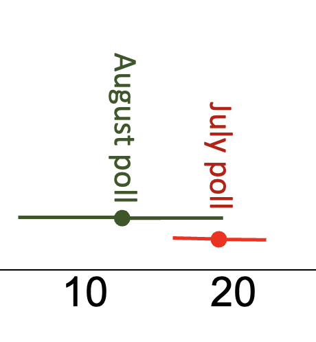
You can see in the figure above that the confidence intervals overlap. Yes, DeSantis could have fallen, but he could also be at the same level of support both times. We don't have support at the 95% confidence level to argue that DeSantis fell from July to August. DeSantis' July and August numbers are not significantly different.
We see these kinds of claims across the media, and among social and political commentators, who get swept up in candidate polling. For example, I remember when former Secretary of Labor Bob Reich put out a Facebook post about a New York Times article that sensationalized the changes from their June to July polls. Check out the post below on the left and then my discussion of it below on the right.
 |
Reich claimed that Clinton went from having a lead among voters in June to being tied in July. But the change was not statistically significant.
Reich also claimed that in July, 5% more voters felt Clinton was not honest or trustworthy compared to June, and then argued that the FBI's report on Clinton's e-mail was the reason for this 5% shift. But this change was also not statistically significant.
Sampling error takes into account that samples are often not exactly representative of their target populations. Taking into account margins of error helps us have a sense of how close we should expect the poll results to be to how the target population would respond to such a poll. Building these confidence intervals shows that there could have been real changes, or it could just be that the July poll's random sample of registered voters liked Clinton less than the sample from June, regardless of the month. Of course, taking into account the polls' margins of errors results in a much less sexy news story --- read the headline now: We're not Sure if Anything Changed This Past Month. |

A Quinnipiac University Poll RDD (random digit dialing) telephone survey of 1,795 U.S. adults, conducted March 9-13, 2013, had a reported margin of sampling error of "+/- 3.0 percentage points."
One poll question asked was, "What is your biggest personal financial concern right now: food costs, healthcare costs, mortgage or rent payments, energy bills, credit card or loan payments, college tuition, retirement savings, or loss of a job?"
According to the release,
Food costs rank as the most pressing financial worry, with 22 percent of Americans naming it as their biggest personal financial concern right now, followed by retirement savings (18 percent), healthcare costs (17 percent), mortgage or rent payments (13 percent), college tuition (8 percent), energy bills (7 percent), credit card or loan payments (5 percent), and loss of a job (4 percent), according to a Quinnipiac (KWIN-uh-pea-ack) University national poll of adults released today.
Significant differences
Among all U.S. adults at the time of the survey, was food the biggest financial concern? Which concerns can we be confident are significantly greater than/less than others among all U.S. adults?
While we know the survey results, we want to know about the concerns of all U.S. adults.
Here are the sample proportions along with confidence intervals. In the table, P is for the sample proportion, LB for lower bound of the confidence interval, and UB for upper bound of the confidence interval:
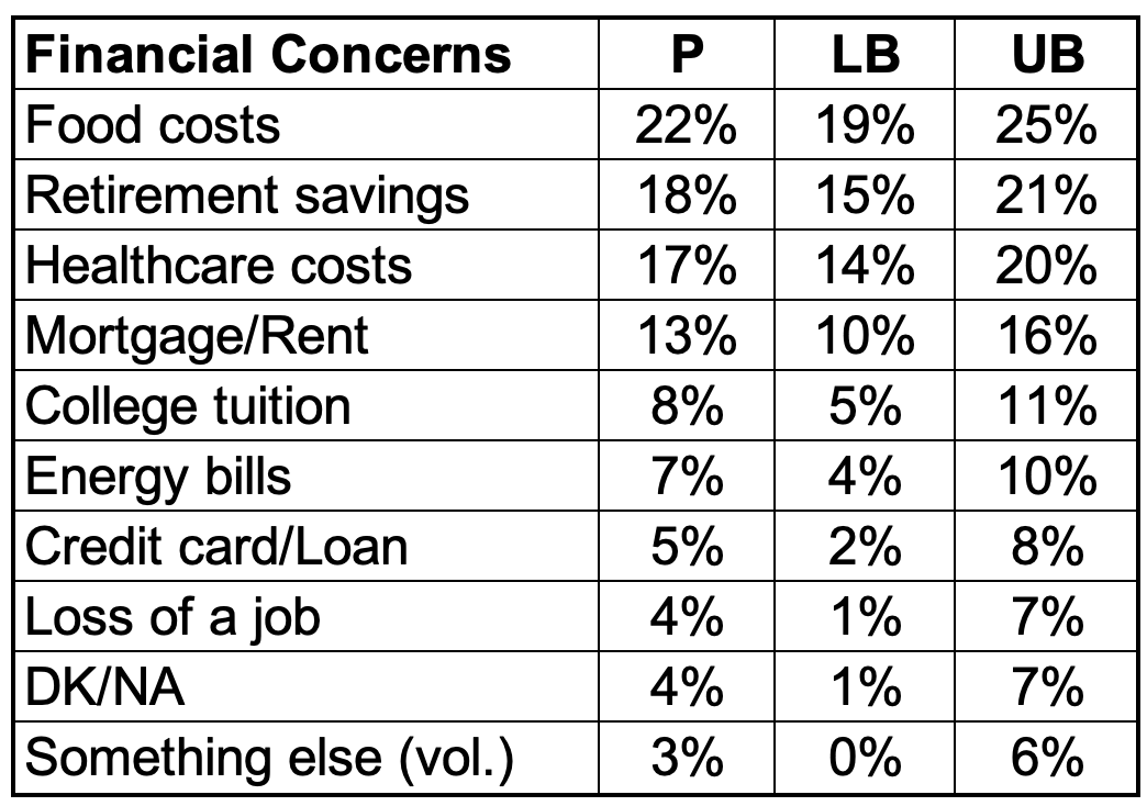
While the headline read that U.S.-Americans are most concerned about food costs, the proportion of U.S. adults concerned about food costs at the time of the survey is not significantly different from the proportion concerned about retirement savings or healthcare costs. We're not sure which of these three takes the top spot. However, we are confident a higher proportion of U.S. adults are most concerned about food costs compared to each of the other five options.
Substantive differences
While evaluating whether something is substantively different involves subjective judgment calls and evaluating differences in context (don't forget to use your codebook!), in general I look for differences that I am 95% confident are at least 5% different or differences where I am 95% confident that the results for two groups have qualitatively different meanings.
- We can be confident that substantively more U.S. adults are most concerned with food costs compared to college tuition, energy bills, credit cards/loans, or loss of a job. While we are confident that somewhere between 19% and 25% of U.S. adults are most concerned with food costs, these other areas are each a top concern for somewhere between 1% and 11% of U.S. adults.
- We can be confident that substantively more U.S. adults are most concerned with retirement savings compared to energy bills, credit cards/loans, or loss of a job. While we are confident that somewhere between 15% and 21% of U.S. adults are most concerned with retirement savings, these other areas are each a top concern for somewhere between 1% and 10% of U.S. adults.
- We can be confident that substantively more U.S. adults are most concerned with health care costs compared to credit cards/loans, or loss of a job. While we are confident that somewhere between 15% and 21% of U.S. adults are most concerned with retirement savings, these other areas are each a top concern for somewhere between 1% and 10% of U.S. adults.
Concerns by Age
The survey release continues,
There are differences among most listed groups, particularly when considering age.
The top three personal financial concerns broken down by age:
- 18 to 34 year olds: mortgage or rent payments (23 percent), college tuition (20 percent), and food costs (19 percent);
- 35 to 49 year olds: food costs (24 percent), retirement savings (17 percent), and mortgage or rent payments (15 percent);
- 50 to 64 year olds: retirement savings (25 percent), food costs (23 percent), and healthcare costs (19 percent);
- 65 years of age and over: retirement savings (26 percent), food costs (22 percent), and healthcare costs (20 percent).
These differences in the narrative were based on sample proportions. Upon request, I received margins of error for the age subgroups: 6.09% for ages 18-34, 5.46% for ages 35-49, 4.46% for ages 50-64, and 3.91% for ages 65+. The table below shows sample proportions and confidence intervals for each age group. Looking at each age group, the yellow highlights are the highest sample proportions for the age group, and the grey-shaded cells are the areas that, for that age group, are not significantly different than the yellow highlights.
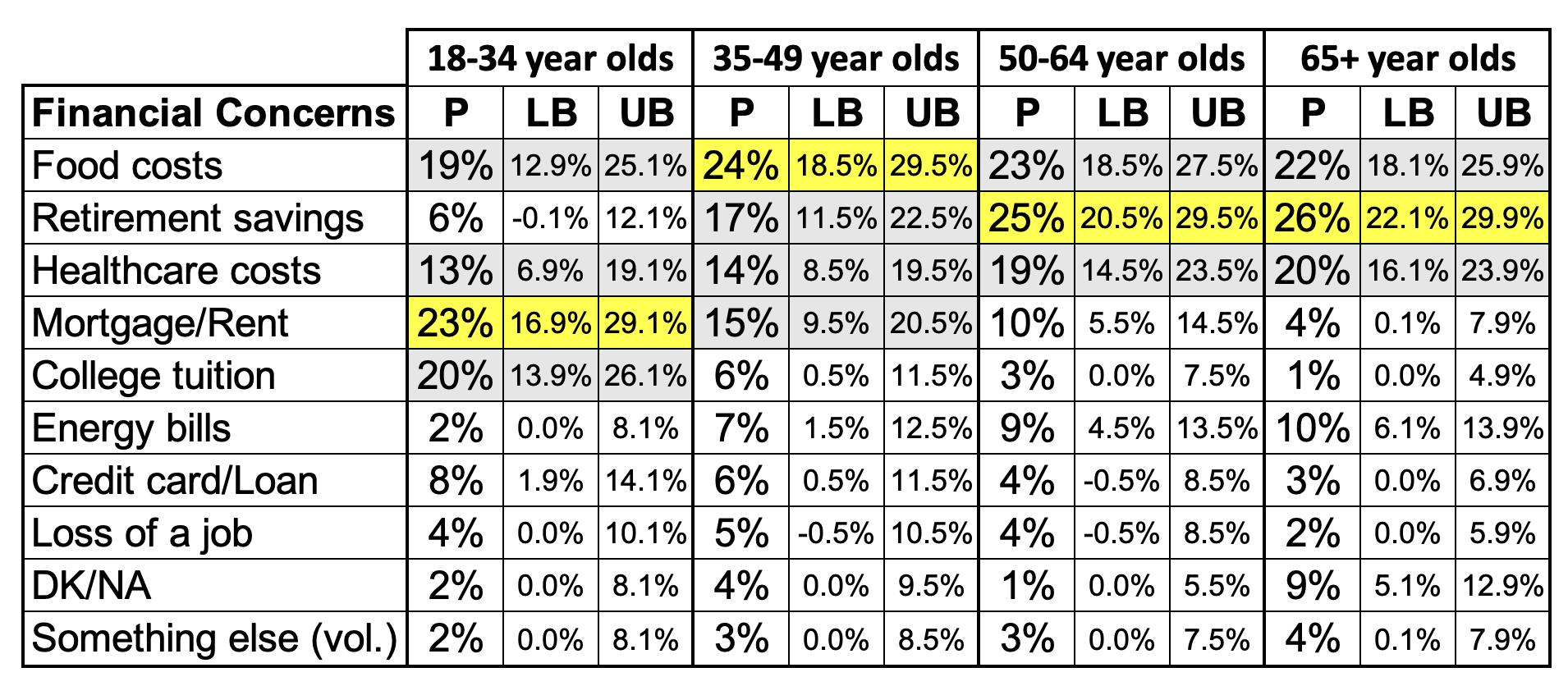
It could be that food costs were the top concern for each age group, though it could also be that food costs were not the top concern for any age group. What is most notable is that mortgage rent is substantially more likely to be a top concern for 18-34 year olds than 65+ year olds, college tuition is substantially more likely to be a top concern for 18-34 year olds than 50-64 and 65+ year olds, and retirement savings is substantially more likely to be the top concern for 50-64 and 65+ year olds compared to 18-34 year olds.
Using Explore/Examine to Examine Relationships
Generating confidence intervals for subgroups is very similar to generating confidence intervals like we did in Chapter 5, but with one extra step (in bold below). This is the same process you used in Chapter 2 to generate comparative statistics and side-by-side box plots for analyzing relationships.
Menu:
Go to: Analyze → Descriptive Statistics → Explore.
Put your variable into the "Dependent List:" window/box.
Put your categorical variable into the "Factor list:" box.
At the bottom where it says "Display," make sure you either have "Both" or "Statistics" checked. (Plots will only give you graphs/figures.)

Syntax:
EXAMINE VARIABLES=PrimaryVariableName BY CategoricalVariableName
/PLOT BOXPLOT
/COMPARE GROUPS
/PERCENTILES(25,50,75) HAVERAGE
/STATISTICS DESCRIPTIVES
/CINTERVAL 95
/MISSING LISTWISE
/NOTOTAL.
In Chapter 5, we found that, at the 95% confidence level, following the 2020 general election, U.S. eligible voters mean feelings thermometer scores towards journalists were somewhere between 49.21° and 51.45°, meaning on average they were neutral or close to neutral in their feelings towards journalists (the average is somewhere between just cooler or warmer than neutral).
Biden vs. Trump
Let's compare feelings towards journalists among those who voted for Biden vs. those who voted for Trump.
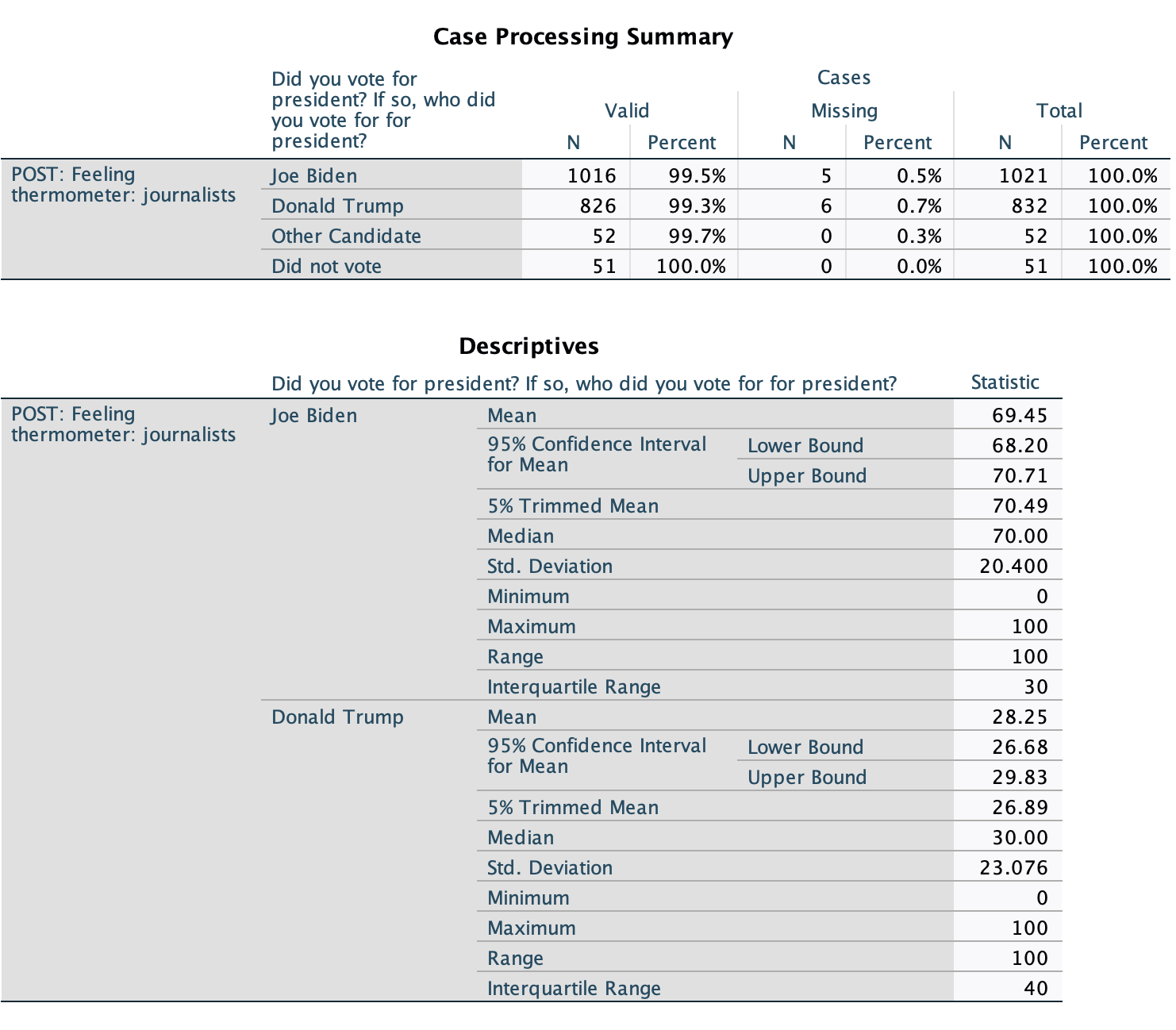
Looking at the sample means, we can see that, among survey respondents who voted for Biden, the mean feeling towards journalists was 69.45 degrees, or about fairly warm/favorable. Among survey respondents who voted for Trump, the mean feeling towards journalists was 28.25 degrees, or about fairly cold/unfavorable. These are 41.2 degrees apart.
As noted, we don't really care about how the survey participants feel, however. We want to know about how all Biden voters and how all Trump voters feel. Here are their confidence intervals: Biden 95% CI: 68.20°, 70.71°; Trump 95% CI: 26.68°, 29.83°
1. Are they significantly different?
Yes! At the 95% confidence level, the warmest Trump voters might be, on average, is 29.83°, and the coldest Biden voters might be, on average, is 68.20°. These do not overlap. We are over 95% confidence that Trump and Biden voters had different mean feelings towards journalists following the 2020 elections.
2. Are they substantively different?
We are 95% confident that Trump and Biden supporters' mean feelings towards journalists are at least 38.37 degrees apart (and could be up to 44.03 degrees apart). (I got these numbers by finding the difference of the closest bounds from each CI to each other, 68.20-29.83, and the further bounds from each CI to each other, 70.71-26.68.) Given how far apart they are, and that we are confident Trump supporters average cold feelings and that Biden supporters average warm feelings, they are substantively different.
3. Do they have a causal relationship?
Next chapter we will discuss causality. Do you think that being a Biden vs. Trump supporter might have an impact on how one feels about journalists? Given Trump's repeated repeated claims that the media is promoting "fake news", I would say it's likely!
Causality / Causation: There is a causal relationship when one variable has an impact or effect on variation of another variable.
Gender
Let's compare feelings towards journalists among men vs. women eligible voters.
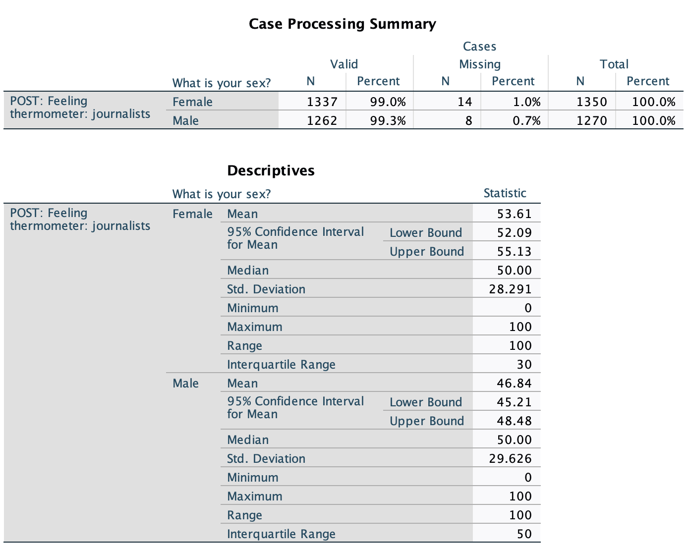
Looking at the sample means, we can see that, among survey respondents, women's mean feelings towards journalists were 53.61°, a tad warmer than neutral, and men's mean feelings towards journalists were 46.84°, a tad colder than neutral.
We don't really care about how the survey participants feel, however. We want to know about all U.S. men and women eligible voters feel.
Here are their confidence intervals: Women 95% CI: 52.09°, 55.13°; Men 95% CI: 45.21°, 48.48°
1. Are they significantly different?
Yes! At the 95% confidence level, the warmest men could be, on average, is 48.48°, and the coldest women could be, on average, is 52.09°. These do not overlap. We are over 95% confidence that men and women eligible voters had different mean feelings towards journalists following the 2020 elections.
2. Are they substantively different?
We are 95% confident that men and women, on average, are at least 3.61 degrees different (and at most 9.92 degrees different). (I got these numbers by finding the difference of the closest bounds from each CI to each other, 52.09-48.48, and the further bounds from each CI to each other, 55.13-45.21.) While these numbers are not that far apart on the 0° to 100° thermometer, given that we are 95% confident women's average leans warm (at least 52.09°) and men's average leans cold (at most 48.48°), this seems substantive to me.
3. Do they have a causal relationship?
Does gender impact variation in how people feel towards journalists? Following the 2020 election, this could make sense, if for no other reason than that, compared to men, women were more supportive of Biden and less supportive of Trump.
Age
Let's compare feelings towards journalists by age.
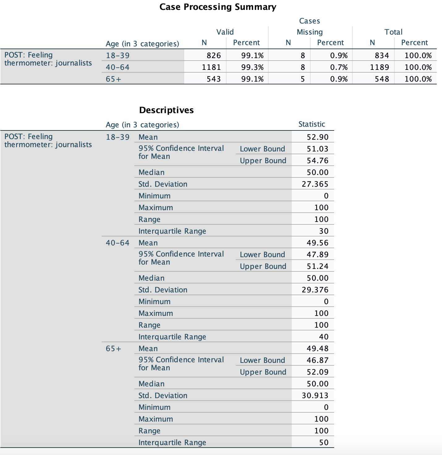
Looking at the sample means, we can see that survey respondents ages 18-39's mean feeling towards journalists was 52.90°, a tad warmer than neutral, survey respondents ages 40-64's mean feeling towards journalists was 49.56°, just a smidgen colder than neutral, and survey respondents ages 65 or older's mean feelings towards journalists was 49.48°, also a smidgen colder than neutral.
We don't really care about how the survey participants feel, however. We want to know about all U.S. eligible voters of these age groups feel on average.
Here are their confidence intervals:
- Ages 18-39: 51.03°, 54.76°
- Ages 40-64: 47.89°, 51.24°
- Ages 65+: 46.87°, 52.09°
1. Are they significantly different?
No! While the youngest age range (18-39) had average warmer feelings in the sample, at the 95% confidence level all the confidence intervals overlap. For example, they could all be at 51 degrees, a smidgen warmer than neutral, in their feelings towards journalists.
2. Are they substantively different?
First, let's look at how different each age group's means might be from one another at the 95% confidence level.
If you're not sure how to solve this, sketch out the confidence intervals above a number line, and then figure out which numbers to subtract.
Ages 18-39 & Ages 40-64: Ages 18-39 could be anywhere from 6.87 degrees warmer (54.76-47.89) to the same (they overlap from 51.03 to 51.24) to 0.21 degrees colder (51.24-51.03) than ages 40-64.
Ages 18-39 & Ages 65+: Ages 18-39 could be anywhere from 7.89 degrees warmer (54.76-46.87) to the same (they overlap from 51.03 to 52.09) to 1.06 degrees colder (52.09-51.03) than ages 65+.
Ages 40-64 & Ages 65+: Ages 40-64 could be anywhere from 4.37 degrees warmer (51.24-46.76) to the same (they overlap from 47.89 to 51.24) to 4.2 degrees colder (52.09-47.89) than ages 65+.
So, are they substantively different?
They could be, e.g., at 95% confidence ages 18-39 could have an average that is 7.89 degrees warmer than ages 65+ (54.76-46.87), with the younger group having warm feelings on average and the older group on average cold feelings. However, we don't have evidence to show this is the case. At the 95% confidence level, ages 65+ could have slightly warmer average feelings than ages 18-39 (e.g., 52.05° vs. 51.05°) or they could have the same average feelings (e.g., both could have a mean of 52°). All three confidence intervals overlap (e.g., all three age groups could have a mean of 51.2°), so at the 95% confidence level, we are not confident they are different at all, let alone by a sizable amount. We will not claim they are substantively different.
3. Are they causal?
Does age impact variation in how people feel towards journalists? Given that no relationship was identified, there cannot be a causal relationship. If age was affecting feelings towards journalists, we would expect to see different age groups have different average feelings towards journalists (barring any suppression effects, but don't worry about that right now).
For our final example, let's look back at the 2022 General Social Survey question asked of U.S. adults, "Have you ever tried to encourage someone to believe in Jesus Christ or to accept Jesus Christ as his or her savior?" This was recoded as an indicator variable (0=no, 1=yes). While the confidence intervals could be interpreted the same as the other examples with interpreting means (e.g., the sample mean in the Mountain region is 0.35; the 95% confidence interval for the Mountain region is 0.29 to 0.41), it makes more sense to interpret them as proportions (e.g., the sample proportion in the Mountain region is 35%, the 95% confidence interval for the Mountain region is 29% to 41%). Rather than comparing means, we're comparing the actual percentages of respondents (sample) or of the target population (in this case U.S. adults) that have the value of 1 (in this case, having engaged in Christian proselytization).
Region
The map below shows, for each region, sample proportions (inner circle) and confidence intervals at the 95% confidence level (lower bounds in middle circle, upper bounds in outer circle), with the peach-colored sectors with the labeled percentages the proportions who answered yes, that they have tried to encourage someone to believe in Jesus Christ or to accept Jesus Christ as their savior.
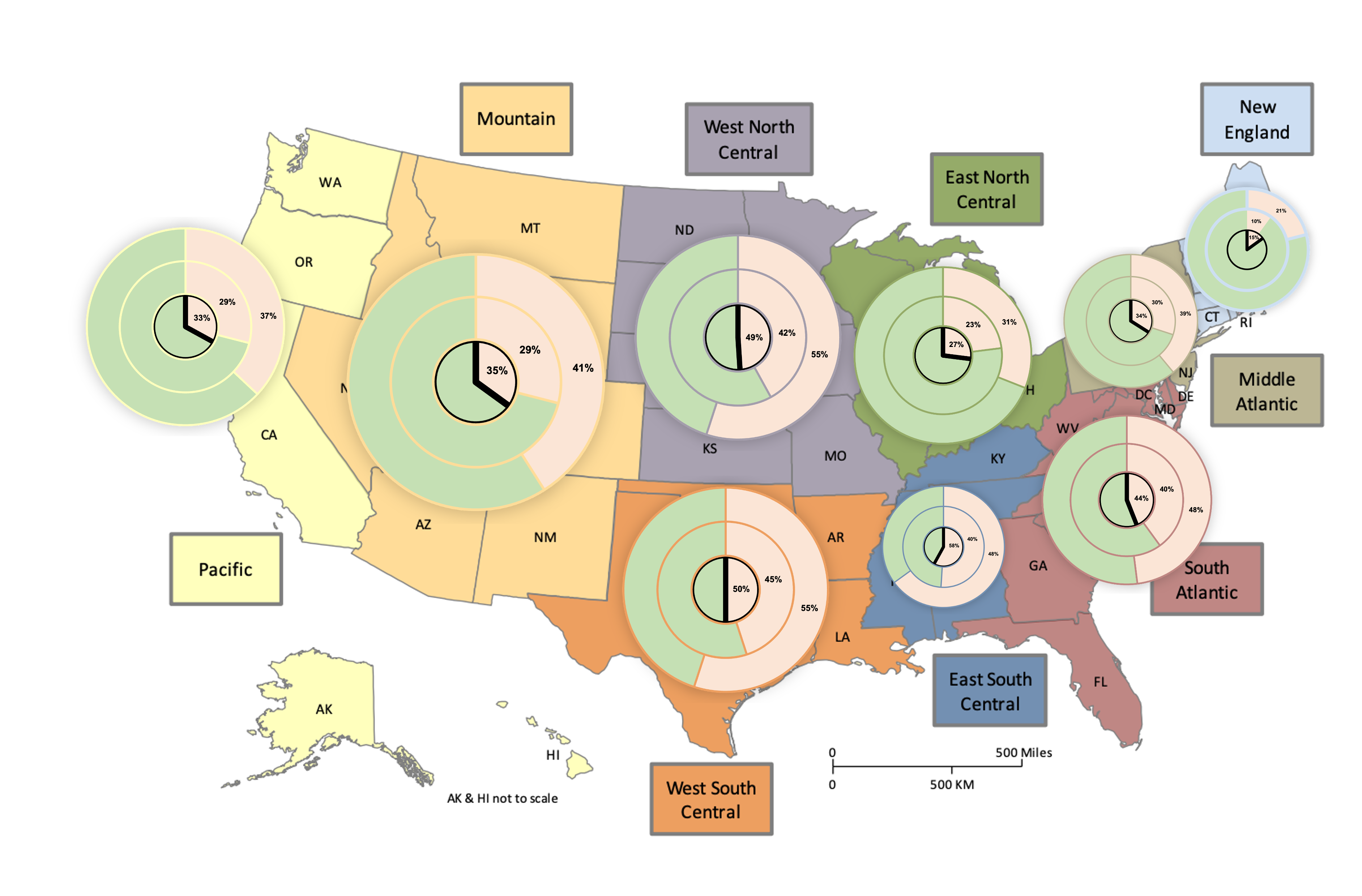
1. Are the regions significantly different?
- Significantly fewer New England adults proselytize for Jesus compared to any other regions, and vice versa. At the 95% confidence level, the maximum proportion of New England adults that have proselytized for Jesus is 21%, whereas all other regions are 23% or higher.
- The Middle Atlantic, East North Central, Pacific, and Mountain regions are not significantly different from one another (e.g., at the 95% confidence level, there could be 29% to 30% of adults in each of these regions that have proselytized for Jesus). They are, however, all significantly higher than New England and significantly lower than the remaining four regions.
- The South Atlantic, West North Central, and West South Central regions are not significantly different from one another (e.g., at the 95% confidence level, there could be 45% to 48% of adults in each of these regions that have proselytized for Jesus).
- The South Atlantic region is significantly lower than the East South Central/Atlantic region, and vice versa (at the 95% confidence level, at most 48% of South Atlantic adults have proselytized for Jesus and at least 51% of East South Central/Atlantic adults have).
- The West North Central, West South Central, and East South Central/Atlantic regions are not significantly different from one another (e.g., at the 95% confidence level, there could be 51% to 55% of adults in each of these regions who have proselytized for Jesus).
2. Are the regions substantively different (at the 95% confidence level)?
Since we are not confident about differences existing between certain regions, we also will not claim those regions have substantively different percentages of their adult residents who have proselytized for Jesus. This means that we do not have evidence that the Middle Atlantic, East North Central, Pacific, or Mountain regions are substantively different from one another, that the South Atlantic, West North Central, and West South Central regions are substantively different from one another, or that the West North Central, West South Central, and East South Central/Atlantic regions are substantively different from one another. Among the regions that are significantly different from one another, we need to evaluate whether those differences are sizable. New England is substantively different from the other seven regions; we are 95% confident New England is at least 8% lower than them (the highest New England could be is 21% and the lowest any of the other seven could be is 29%).
- The East North Central and Pacific regions are both substantively different from the South Atlantic, West North Central, West South Central, and East South Central/Atlantic regions. At the 95% confidence level, the East North Central region is at maximum 31% and Pacific region at maximum 33%, while the other four named regions are all at least 40% or higher.
- The Mountain region and Middle Atlantic region are substantively less than the East South Central/Atlantic region. At the 95% confidence level, the Mountain region is at most 41% and the Middle Atlantic region at most 39%, and these are meaningfully less than the East South Central/Atlantic region which is at least 51%.
- The Middle Atlantic region is also substantively less than the West South Central region, as they are at least 5% different, so at least 1/20 more adults in West South Central have proselytized compared to the Middle Atlantic region.
- We cannot be confident, at the 95% confidence level, that any other regions are 5% or more different from one another. For example, while New England is significantly lower than East North Central, and it might be substantively different (e.g., New England could be at 10% and East North Central at 31%), we are only 95% confident that New England and East North Central are at least 2% different (New England could be at 21% and East North Central at 23%). We do not have evidence to claim they are substantively different.
3. Is there a causal relationship?
The regions with more proselytizing are more religious and have a higher proportion of evangelical Christian residents. These factors could impact proselytizing rates.
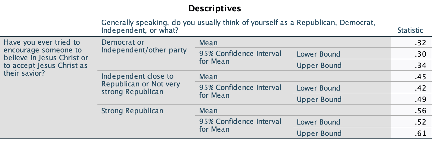
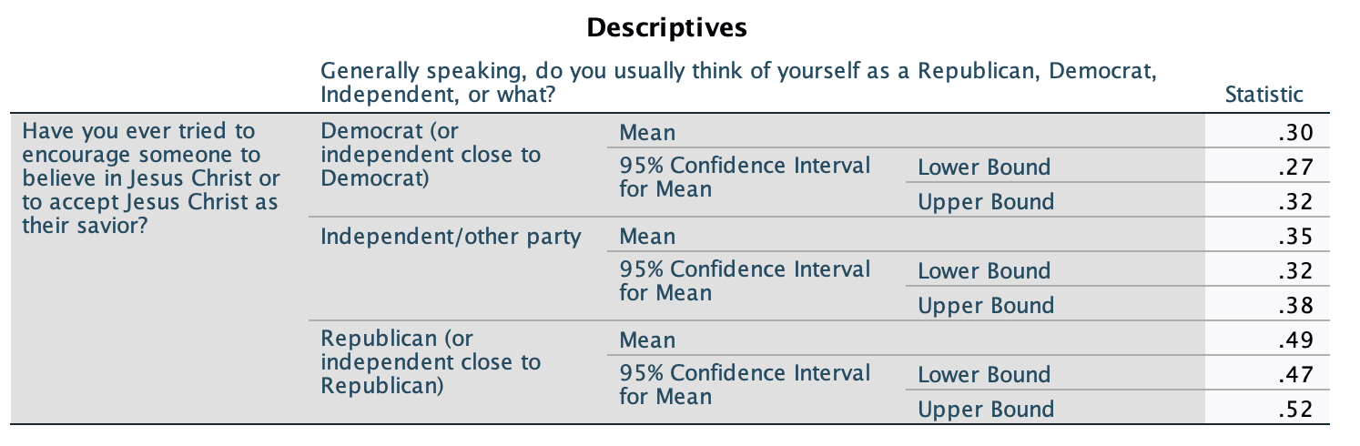
Political Party
The graph below shows sample proportions along with 95% confidence intervals of those who said they have engaged in Christian proselytization, broken down by self-reported political party identification.
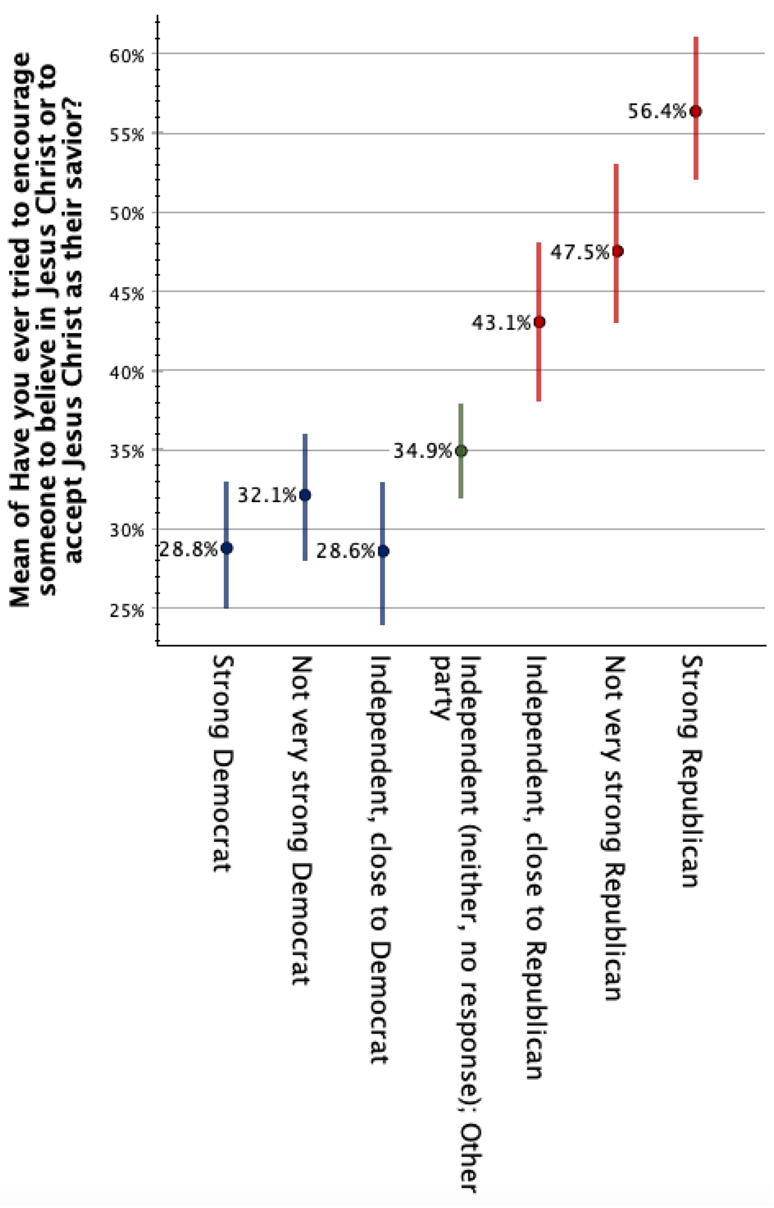
The graph is based on these confidence intervals:
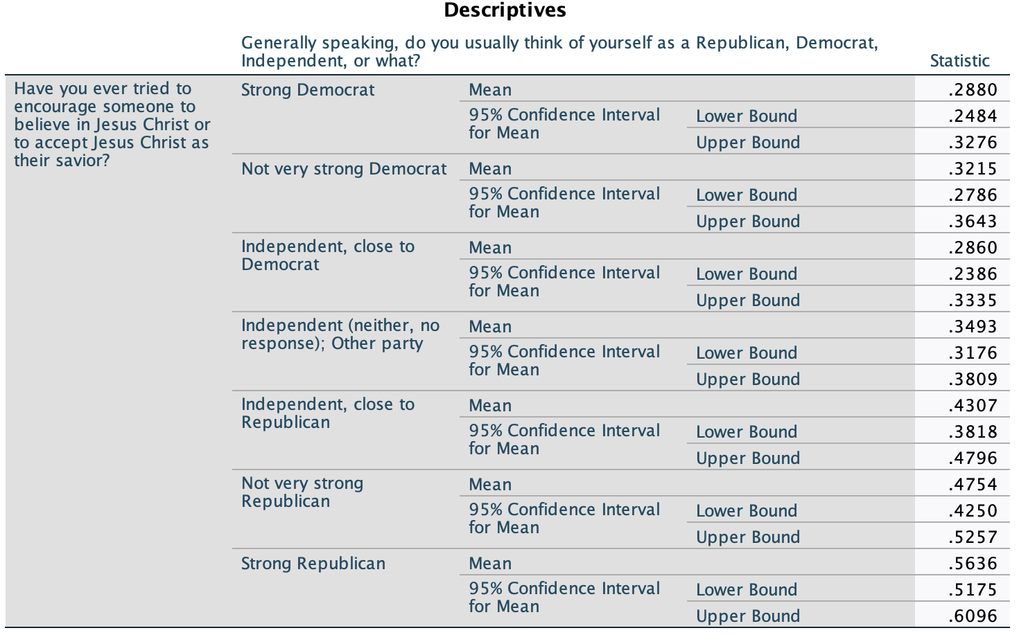
1. Are the parties significantly different?
Looking at the graph above, you can see which confidence intervals do and do not overlap. (The one exception is Independents/Other Party and Independents close to Republicans, as they are too close to tell, but they do not overlap --- they are 0.09% apart.)
- Strong Democrats, not very strong Democrats, Independents close to Democrats, and Independents are all not significantly different from one another. At the 95% confidence level, they could all be anywhere between 31.76% and 32.76%, and the first three Democratic or Democratic leaning groups could all be between 27.87% and 32.76%.
- These four groups are all significantly different from Independents close to Republicans, not very strong Republicans, and strong Republicans. At the 95% confidence level, the most any of the first three groups could be is 36.43%, the most the Independents group could be is 38.09%, and the least any of the last three Republican or Republican leaning groups could be is 38.18%.
- Independents close to Republicans are not significantly different from not very strong Republicans. At the 95% confidence level, they both could be between 42.5% and 47.96%.
- Independents close to Republicans are significantly different from strong Republicans. At the 95% confidence level, Independents close to Republicans are at most 47.96%, while strong Republicans are at least 51.75%.
- Not very strong Republicans and strong Republicans are not significantly different from each other. At the 95% confidence level, they could both be between 51.75% and 52.57%.
2. Are the parties substantively different?
We cannot claim that any groups that are not significantly different are substantively different. They could be, e.g., at the 95% confidence level, it could be that less than 1/4 of strong Democrats proselytize (24.84%) while over 1/3 of not very strong Democrats proselytize (36.43%), but these two groups could be identical, e.g., it could be that 3/10 of both groups proselytize.
Among the groups that are significantly different, let's explore whether we can be confident at the 95% confidence level that they are substantively different.
- Strong Democrats are substantively different from Independents close to Republicans (at least 5.4% lower), not very strong Republicans (at least 9.7% lower), and strong Republicans (at least 19.0% lower).
- Not very strong Democrats are substantively different from not very strong Republicans (at least 6.1% lower) and strong Republicans (at least 15.3% lower).
- Independents closer to Democrats are also substantively different from not very strong Republicans (at least 9.2% lower) and strong Republicans (at least 18.4% lower).
- Independents are substantively different from strong Republicans (at least 13.7% lower).
- All other groups could be less than 5% different, at the 95% confidence level. While other groups might be substantively different from one another (e.g., Independents and not very strong Republicans could be 20.81% different), we do not not have sufficient evidence to claim that they are.
3. Does party have a causal effect on Christian proselytizing?
Perhaps there are differences by party with respect to respecting difference, inclusion, and ethnocentrism. However, it also could be that party is not impacting proselytization, but different religious beliefs and traditions (atheist/agnostic, non-Christian, Christian but not evangelical, Christian evangelical) impact both political party and proselytization in the same direction.
Remember that confidence intervals' widths vary based on sample size, as well as the extent of uniformity/variability within the data for that particular category. Here are confidence intervals of the same data, but this time: 1) party collapsed into three categories, Democrats, Independents, and Republicans, and 2) party collapsed into three categories based on levels of proselytization, Democrats/Independents, weak Republicans, and strong Republicans.
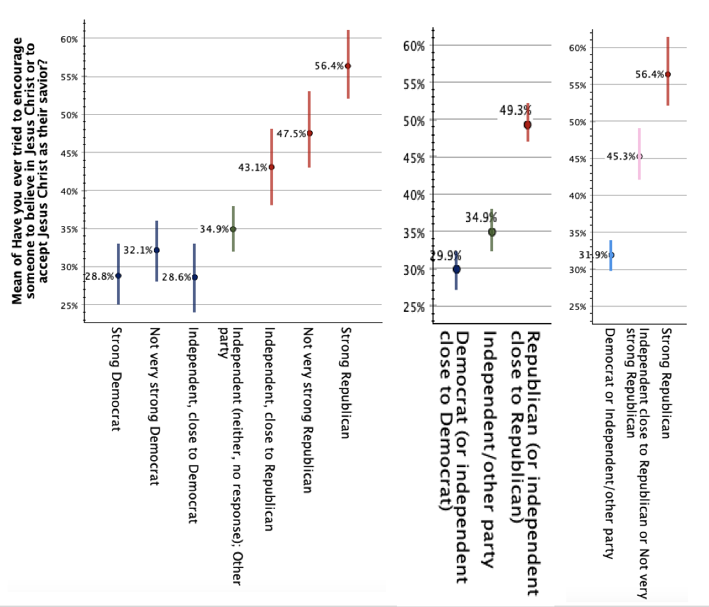
This all comes from the same data, but what do you notice when you compare the graphs? What stories do they tell? Do they tell the same story? Are there differences in what is or is not substantively different, or the extent to which it appears different? If you were to communicate the story of this data, which graph would you choose?
The graph above exaggerates differences, because the y-axis scale goes from 23% to 62%. While zooming in allows you to see differences more closely, it also makes them appear more pronounced than they actually are. Here's the same data, graphed with a y-axis scale from 0% to 100%.
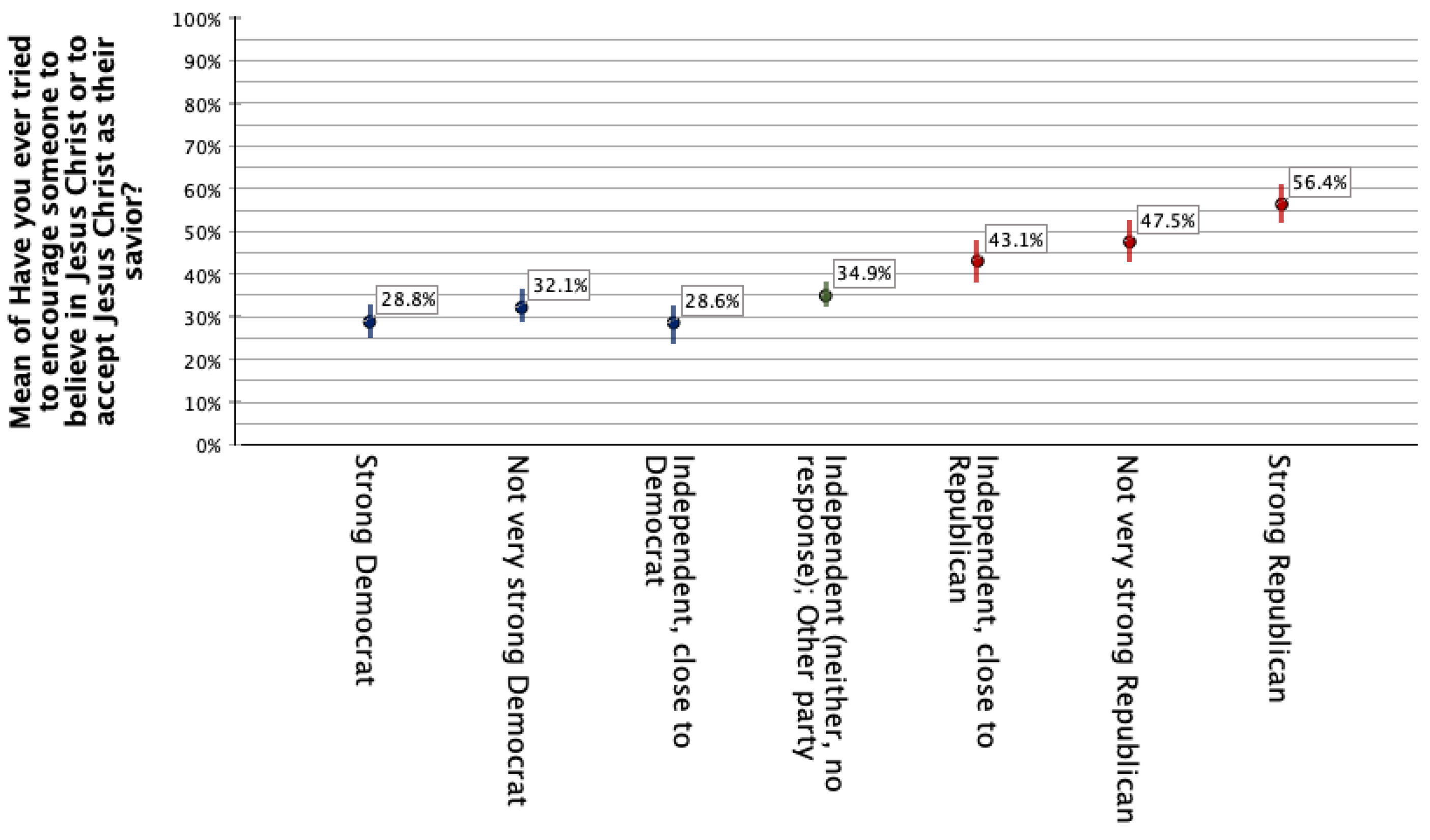
On the one hand, we don't want to exaggerate differences. Are Independent close to Republican and not very strong Republicans really that different from strong Republicans? Their sample means are 11% apart, and at the 95% confidence level they could be 19% apart, but also at the 95% confidence level, they could be only 3% apart (49% and 52%), with about half of people in each group having engaged in Christian proselytization. If these were the numbers, for every 100 people, you would have 49 who did proselytize in the both groups, 48 who did not in both groups, and then the difference would be among the final 3 out of 100 people. However, you also do not want to dismiss these differences. When we are dealing with sample proportions and means, differences can appear smaller than they are. 3% of strong Republicans constitute over 1 million U.S. adults and 3% of independents close to Republican or not very strong Republicans constitute over 1½ million adults. That is a lot more/fewer people who have/have not proselytized.