
8: Crosstabs and Chi-square
- Page ID
- 189028

\( \newcommand{\vecs}[1]{\overset { \scriptstyle \rightharpoonup} {\mathbf{#1}} } \)
\( \newcommand{\vecd}[1]{\overset{-\!-\!\rightharpoonup}{\vphantom{a}\smash {#1}}} \)
\( \newcommand{\dsum}{\displaystyle\sum\limits} \)
\( \newcommand{\dint}{\displaystyle\int\limits} \)
\( \newcommand{\dlim}{\displaystyle\lim\limits} \)
\( \newcommand{\id}{\mathrm{id}}\) \( \newcommand{\Span}{\mathrm{span}}\)
( \newcommand{\kernel}{\mathrm{null}\,}\) \( \newcommand{\range}{\mathrm{range}\,}\)
\( \newcommand{\RealPart}{\mathrm{Re}}\) \( \newcommand{\ImaginaryPart}{\mathrm{Im}}\)
\( \newcommand{\Argument}{\mathrm{Arg}}\) \( \newcommand{\norm}[1]{\| #1 \|}\)
\( \newcommand{\inner}[2]{\langle #1, #2 \rangle}\)
\( \newcommand{\Span}{\mathrm{span}}\)
\( \newcommand{\id}{\mathrm{id}}\)
\( \newcommand{\Span}{\mathrm{span}}\)
\( \newcommand{\kernel}{\mathrm{null}\,}\)
\( \newcommand{\range}{\mathrm{range}\,}\)
\( \newcommand{\RealPart}{\mathrm{Re}}\)
\( \newcommand{\ImaginaryPart}{\mathrm{Im}}\)
\( \newcommand{\Argument}{\mathrm{Arg}}\)
\( \newcommand{\norm}[1]{\| #1 \|}\)
\( \newcommand{\inner}[2]{\langle #1, #2 \rangle}\)
\( \newcommand{\Span}{\mathrm{span}}\) \( \newcommand{\AA}{\unicode[.8,0]{x212B}}\)
\( \newcommand{\vectorA}[1]{\vec{#1}} % arrow\)
\( \newcommand{\vectorAt}[1]{\vec{\text{#1}}} % arrow\)
\( \newcommand{\vectorB}[1]{\overset { \scriptstyle \rightharpoonup} {\mathbf{#1}} } \)
\( \newcommand{\vectorC}[1]{\textbf{#1}} \)
\( \newcommand{\vectorD}[1]{\overrightarrow{#1}} \)
\( \newcommand{\vectorDt}[1]{\overrightarrow{\text{#1}}} \)
\( \newcommand{\vectE}[1]{\overset{-\!-\!\rightharpoonup}{\vphantom{a}\smash{\mathbf {#1}}}} \)
\( \newcommand{\vecs}[1]{\overset { \scriptstyle \rightharpoonup} {\mathbf{#1}} } \)
\(\newcommand{\longvect}{\overrightarrow}\)
\( \newcommand{\vecd}[1]{\overset{-\!-\!\rightharpoonup}{\vphantom{a}\smash {#1}}} \)
\(\newcommand{\avec}{\mathbf a}\) \(\newcommand{\bvec}{\mathbf b}\) \(\newcommand{\cvec}{\mathbf c}\) \(\newcommand{\dvec}{\mathbf d}\) \(\newcommand{\dtil}{\widetilde{\mathbf d}}\) \(\newcommand{\evec}{\mathbf e}\) \(\newcommand{\fvec}{\mathbf f}\) \(\newcommand{\nvec}{\mathbf n}\) \(\newcommand{\pvec}{\mathbf p}\) \(\newcommand{\qvec}{\mathbf q}\) \(\newcommand{\svec}{\mathbf s}\) \(\newcommand{\tvec}{\mathbf t}\) \(\newcommand{\uvec}{\mathbf u}\) \(\newcommand{\vvec}{\mathbf v}\) \(\newcommand{\wvec}{\mathbf w}\) \(\newcommand{\xvec}{\mathbf x}\) \(\newcommand{\yvec}{\mathbf y}\) \(\newcommand{\zvec}{\mathbf z}\) \(\newcommand{\rvec}{\mathbf r}\) \(\newcommand{\mvec}{\mathbf m}\) \(\newcommand{\zerovec}{\mathbf 0}\) \(\newcommand{\onevec}{\mathbf 1}\) \(\newcommand{\real}{\mathbb R}\) \(\newcommand{\twovec}[2]{\left[\begin{array}{r}#1 \\ #2 \end{array}\right]}\) \(\newcommand{\ctwovec}[2]{\left[\begin{array}{c}#1 \\ #2 \end{array}\right]}\) \(\newcommand{\threevec}[3]{\left[\begin{array}{r}#1 \\ #2 \\ #3 \end{array}\right]}\) \(\newcommand{\cthreevec}[3]{\left[\begin{array}{c}#1 \\ #2 \\ #3 \end{array}\right]}\) \(\newcommand{\fourvec}[4]{\left[\begin{array}{r}#1 \\ #2 \\ #3 \\ #4 \end{array}\right]}\) \(\newcommand{\cfourvec}[4]{\left[\begin{array}{c}#1 \\ #2 \\ #3 \\ #4 \end{array}\right]}\) \(\newcommand{\fivevec}[5]{\left[\begin{array}{r}#1 \\ #2 \\ #3 \\ #4 \\ #5 \\ \end{array}\right]}\) \(\newcommand{\cfivevec}[5]{\left[\begin{array}{c}#1 \\ #2 \\ #3 \\ #4 \\ #5 \\ \end{array}\right]}\) \(\newcommand{\mattwo}[4]{\left[\begin{array}{rr}#1 \amp #2 \\ #3 \amp #4 \\ \end{array}\right]}\) \(\newcommand{\laspan}[1]{\text{Span}\{#1\}}\) \(\newcommand{\bcal}{\cal B}\) \(\newcommand{\ccal}{\cal C}\) \(\newcommand{\scal}{\cal S}\) \(\newcommand{\wcal}{\cal W}\) \(\newcommand{\ecal}{\cal E}\) \(\newcommand{\coords}[2]{\left\{#1\right\}_{#2}}\) \(\newcommand{\gray}[1]{\color{gray}{#1}}\) \(\newcommand{\lgray}[1]{\color{lightgray}{#1}}\) \(\newcommand{\rank}{\operatorname{rank}}\) \(\newcommand{\row}{\text{Row}}\) \(\newcommand{\col}{\text{Col}}\) \(\renewcommand{\row}{\text{Row}}\) \(\newcommand{\nul}{\text{Nul}}\) \(\newcommand{\var}{\text{Var}}\) \(\newcommand{\corr}{\text{corr}}\) \(\newcommand{\len}[1]{\left|#1\right|}\) \(\newcommand{\bbar}{\overline{\bvec}}\) \(\newcommand{\bhat}{\widehat{\bvec}}\) \(\newcommand{\bperp}{\bvec^\perp}\) \(\newcommand{\xhat}{\widehat{\xvec}}\) \(\newcommand{\vhat}{\widehat{\vvec}}\) \(\newcommand{\uhat}{\widehat{\uvec}}\) \(\newcommand{\what}{\widehat{\wvec}}\) \(\newcommand{\Sighat}{\widehat{\Sigma}}\) \(\newcommand{\lt}{<}\) \(\newcommand{\gt}{>}\) \(\newcommand{\amp}{&}\) \(\definecolor{fillinmathshade}{gray}{0.9}\)In this chapter we will evaluate relationships between two categorical variables. We will use crosstabulation tables for descriptive statistics and chi-square for inferential statistics.
Introduction to Crosstabs
This section will introduce you to crosstabulations.
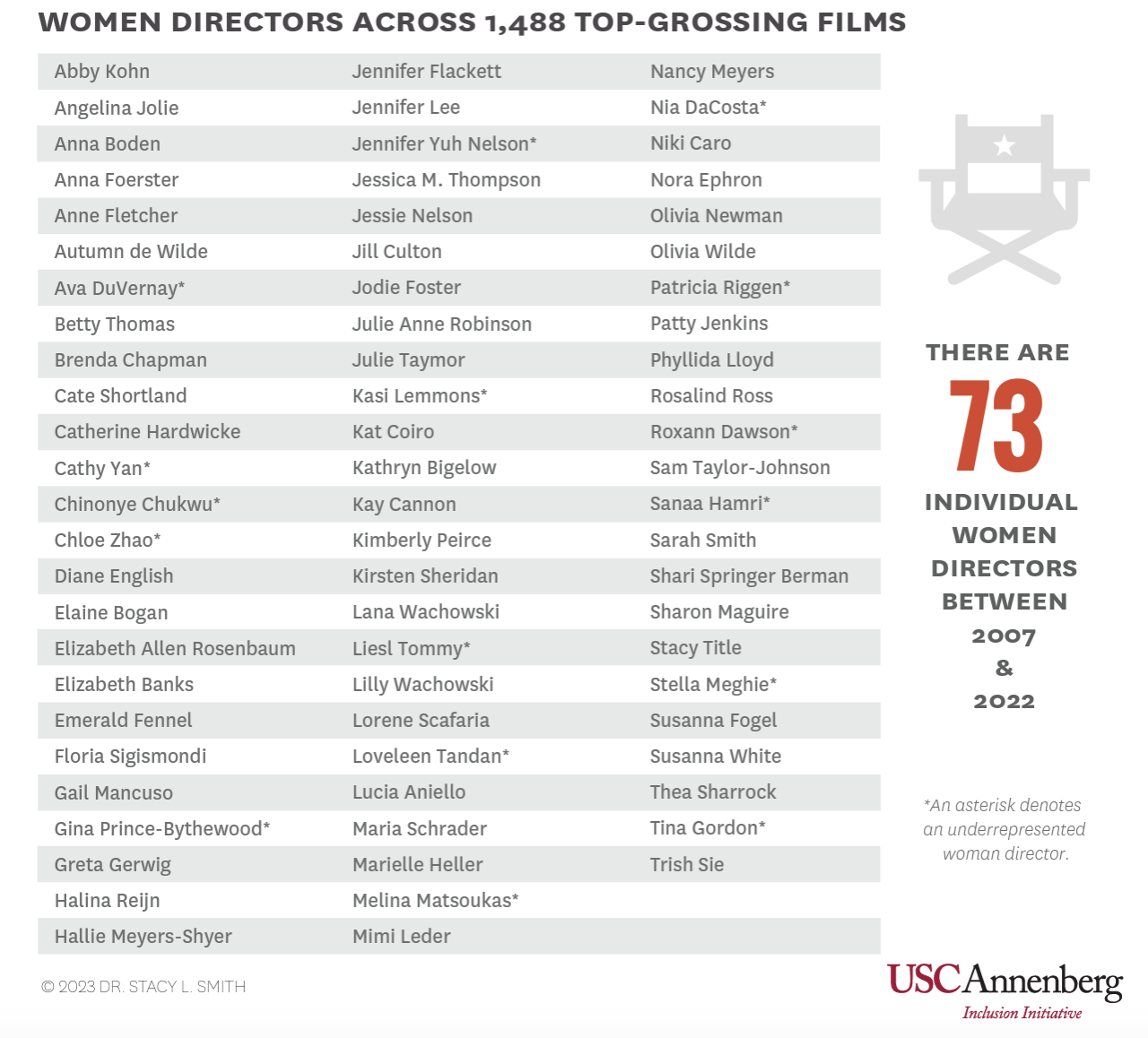
In Chapter 1, you saw an example of frequency tables from a USC Annenberg Inclusion Initiative report by Stacy L. Smith, Katherine Pieper, and Sam Wheeler with an intersectional analysis of gender and race for directors of the 100 top-grossing domestic fictional films in North America from 2007 to 2022 (fewer films were included in 2020 and 2021 due to pandemic-related performance).
Let's take a look at their report on "Inclusion in the Director's Chair." As part of the data collection and analysis, the institute collected a list of directors for each of the 1,488 films, and classified them by gender:
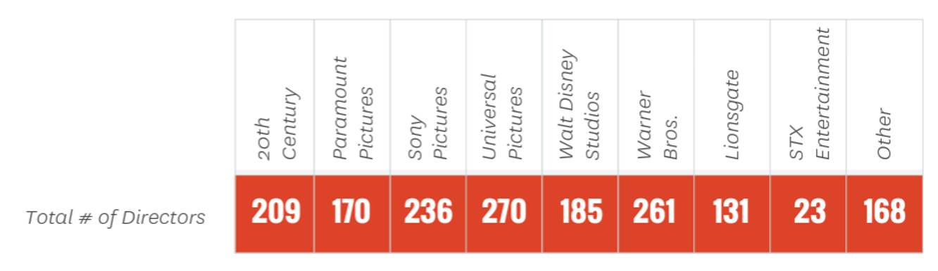
They also classified directors by studio:
What if you wanted to know if there is a relationship between studio and the proportion of women directors? Do some studios do a better or worse job when it comes to women's representation in directing their top films?
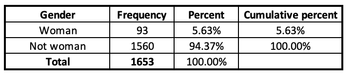
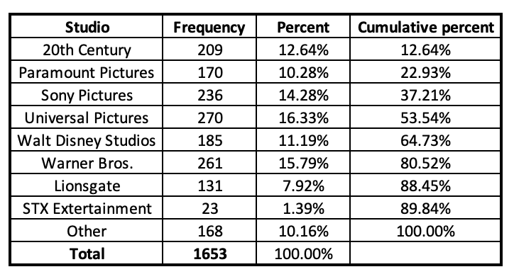
Here are the frequency tables we have for both variables:
Directors by Gender
Directors by Studio
So, is there a relationship? We can't answer this question with the data above. To find out the relationship, we need to be able to go back to the raw data so that we can determine gender breakdown by studio. If there was no relationship / differences, we would expect all the studios to have the same proportion of women directors---we would expect 5.63% of directors in each studio to be women (just over 1/20). However, that's not the case.
Going back to the raw data, we can make a new table of directors that crosses gender and studio. For example, Jennifer Lee and Chris Buck were co-directors for Frozen II in 2019, which was a Walt Disney Studios production. Here you can see the USC Annenberg Inclusion Initiative's table of studios again, but this time they have counted how many of directors within each studio are women.
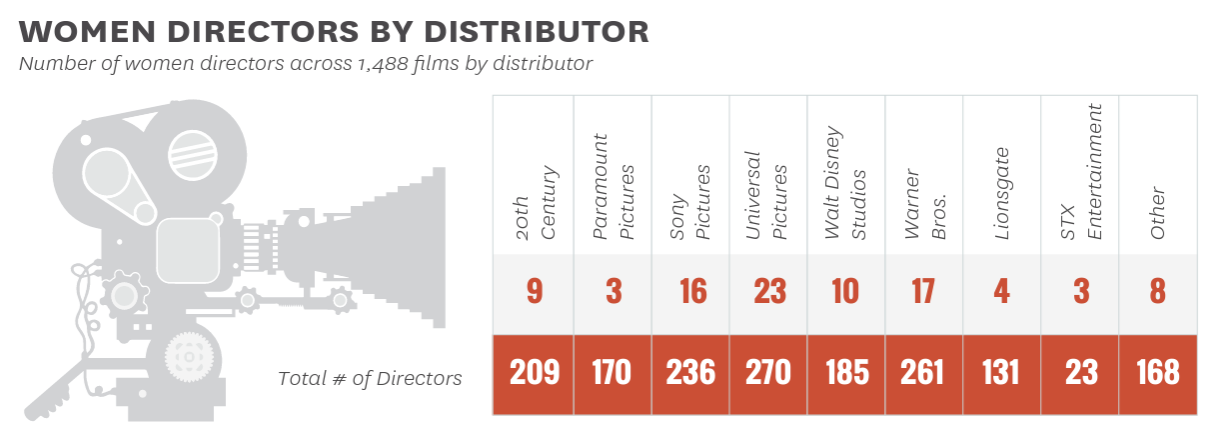
So, are some studios doing better when it comes to women's representation? Universal Pictures has the most women directors, but it also has the most films. Paramount Pictures and STX Entertainment have the fewer women directors, but over 13% (over 1/10) of STX Entertainment directors were women, and 1.8% (under 1/50) of Paramount Pictures directors were women. It's hard to compare studios using frequencies, because the studios do not have an equal number of films.
To make comparisons, we can calculate the percent of directors that are women for each studio.

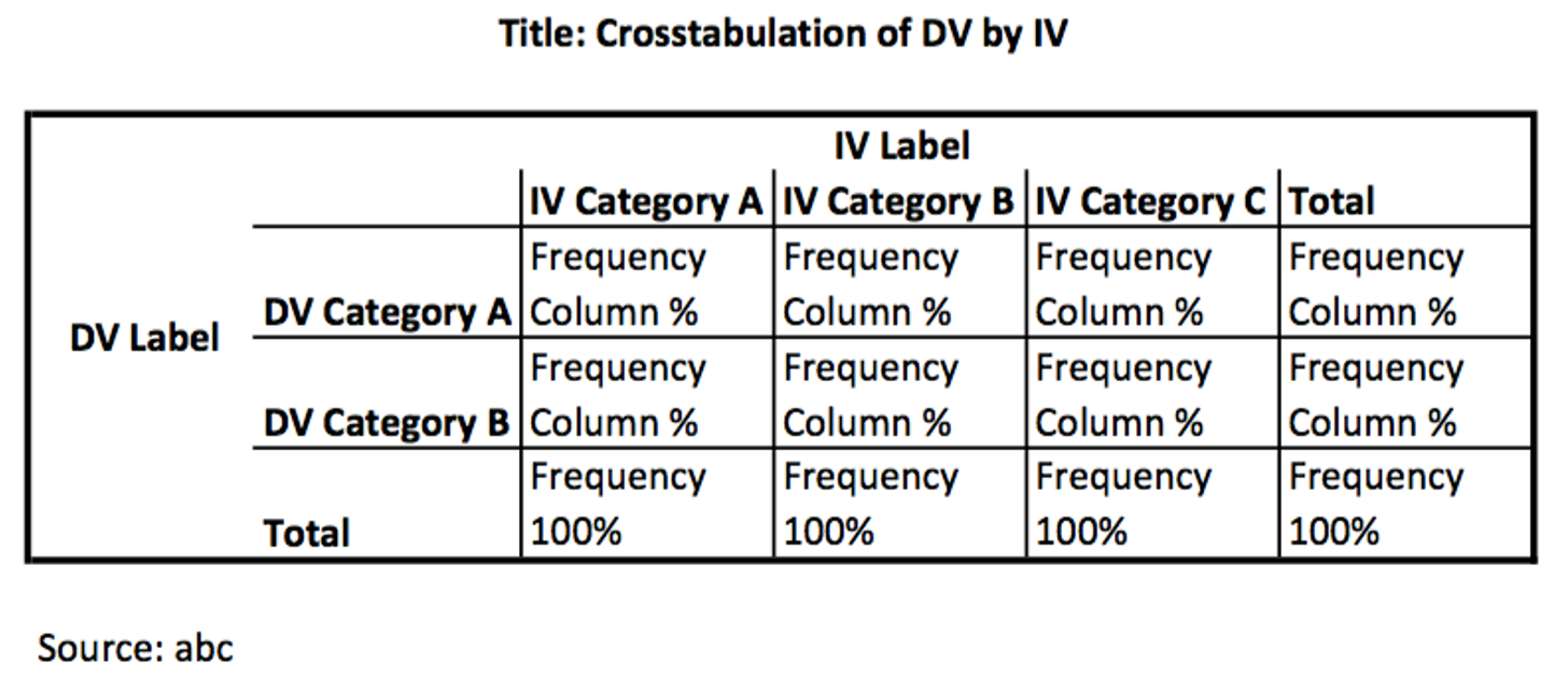
This table is called a crosstabulation, or crosstab for short. It can also be called a contingency table. It tabulates (count up systematically and arranges in table form) our data across two variables.
A crosstabulation, or crosstab, is a table that shows subgroup distribution of data, enabling examination of potential relationships between variables.
When I look at the percent of women by studio, I can make comparisons, going across the row and comparing how similar or different the percentages are. Here we can see that STX Entertainment actually has the highest proportion of women directors, at 13%, and Paramount Pictures the lowest proportion, at 1.8%. Universal Pictures has the second highest proportion of women directors, at 8.5% (over 1/12), and Lionsgate has the second lowest proportion, at 3.1% (about 3/100).
Conversely I could compare the percent of directors that are men, though with a dichotomous variable (there were no non-binary directors), this will just be the inverse of the above, e.g., 87.0% of STX directors were men compared to Paramount with 98.2% men directors. Still, before I give an award to STX Entertainment, I might want to be cognizant that they did not have that many films, comparatively (1.4% of all directors). Because their total number of directors is 23, if just one woman director had instead been a man, they would have dropped to below 9% (though still the highest proportion!), or if just one man director had instead been a woman, they would have jumped up to over 17%. Percentages can fluctuate a lot more with smaller sample sizes, something to be cognizant of when you are comparing percentages.
Later in this chapter we'll discuss chi-square, a statistical test related to crosstabs. For this data, we would not conduct any inferential statistics. This is already population data, containing all of the top-100 grossing films from each year. It's also not a representative sample of all films --- the top-grossing films might be different from other films in terms of who directs them. To consider this a representative sample, each film out of all the films we are interested in would have had to have an equal chance of being included.
Note that the percentages in the table above are column percentages. I wanted to look at whether studio has an effect on women's representation. Studio is my independent variable and gender is my dependent variable. I needed to look at the percent of women directors within each studio. My independent variable is represented in the columns and my dependent variable in the rows.
This is what the table would have looked like with row percentages: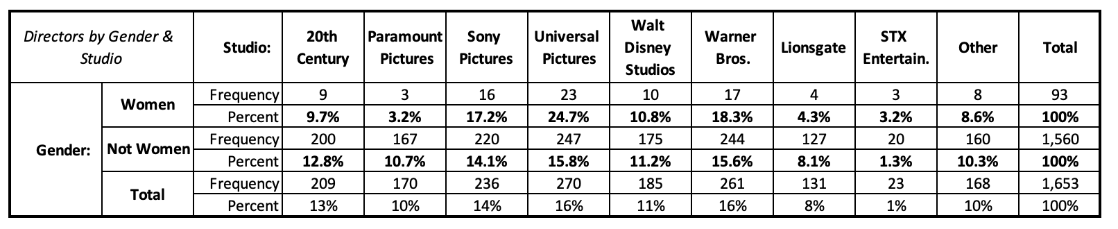
If I had instead used row percentages and compared them, I would have mistakenly thought Universal Studios had the highest proportion of women directors out of any studio! They don't, but because they have the most movies (and the second highest proportion of women directors), they have the highest proportion of women directors out of all women directors. Almost 1/4 of women directors from these top 1,488 films were from Universal Studios.
You will see crosstabs in a variety of formats. Oftentimes in journal articles multiple crosstabs will be combined into one table, and they may not give redundant information (e.g., if they give the percent of women directors, they might not give the percent of directors who are not women). In the infographic above from the report, only frequencies and not percentages were given, and the number of non-women directors was left out.
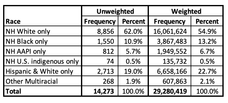
Here is another table from the USC Annenberg Inclusion Initiative's report, this one focused on representation of historically marginalized racial and ethnic groups.
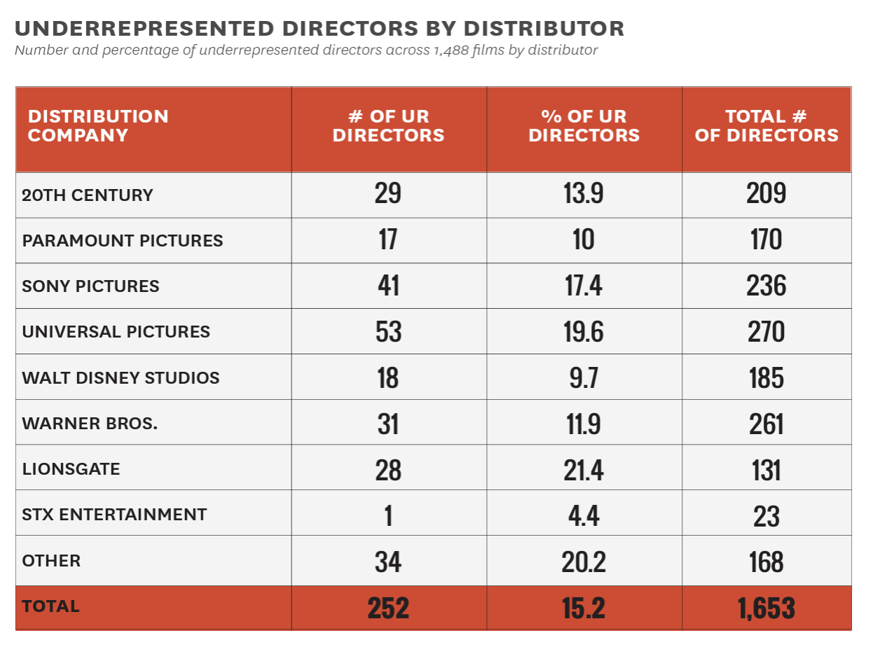
Here there are frequencies and percentages for underrepresented directors, no frequencies or percentages for white directors, and then frequencies for the total number of directors. This table uses row percentages, with the independent variable represented in the rows and the dependent variable in the columns.
While crosstabs can be displayed in a variety of ways, we will use a standard convention in setting ours up, which will allow us to have the information we need in the table and have a consistent method to analyze them. For our tables, the independent variable will be on top, displayed in the columns, and the dependent variable will be on the side, displayed in the rows. We will include both counts and column percentages. Column percentages are the percent of the count for that cell out of the total for that column (for that independent variable category/subgroup).
For example, if we wanted to look at how women directors among these top films are distributed by studio, and our independent variable was gender and dependent variable studio, instead of the table above with row percentages, we would put gender on the top, studio on the side, and use column percentages. The table below shows this, with percentages out of gender. Out of all women directors, how are they distributed by studio?
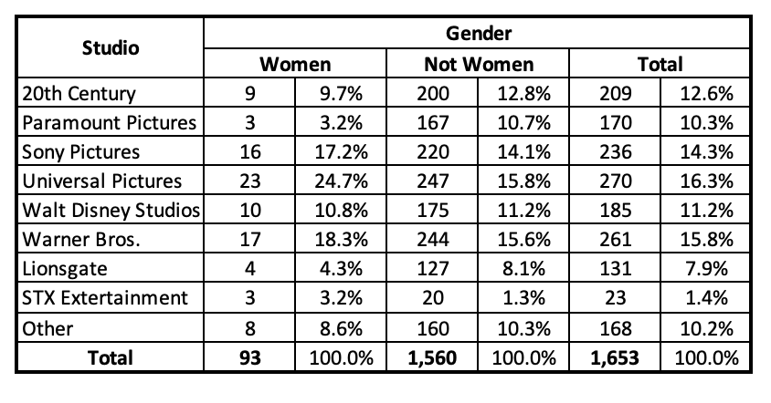
Here we can view the percent of total women directors that come from each studio. Comparing the column percentages as we go across the row, we can also see that some studios are making relatively similar proportional contributions to the totals for women directors and men directors (e.g., Walt Disney Studios has about 11% of all women directors and 11% of all men directors), while others are making differential contributions (e.g., Paramount Pictures had 3.2% of all women directors but 10.7% of all men directors).
Crosstabs are important for us to be able to analyze relationships. When you read poll results or analyze summary statistics by variable, you cannot compare relationships unless you are also given this information already broken down for you or have the raw data and can analyze it yourself. This chapter will teach you how to make crosstabs from a dataset.
Crosstabs is useful when you want to compare two categorical variables. Note that in the analysis above, there were 9 studios and 2 genders. The 9th studio was actually a conglomerate catch-all, "other." You want to use crosstabs when you have a limited number of categories. What if there were 100 different studios included? That would have been a really long table and make comparisons difficult. You can use variables with a lot of categories if you are making a reference table (e.g., if you want to compare all 50 states and D.C., or all countries in the world), but in general you will want variables with a small number of categories. For example, if you wanted to use age and have data with adults, having every year from 18 to 89+ is going to be a big table that will also obscure patterns. Instead, you would want to use a variable that has age in categories (e.g., 18-35, 40-64, 65+). If you are using a ratio-level variable like number of siblings, you would likely want to have an upper cut-off like how the above report used "other" for studios, for example "5 or more siblings." If a table looks overwhelming or you have a number of column totals close to 0 (categories with a very low sample size), you may want to consider collapsing variables into fewer categories.
In this section you'll learn how to run a crosstab and chi-square using SPSS, and also learn about what chi-square is.
This section uses data from the National Crime Victimization Survey's School Crime Supplement, collected by the U.S. Census Bureau in 2019. The sample is representative of its target population, U.S. primary or secondary education (K-12) students ages 12 to 18. Students in private schools were included, but home-schooled children were not. The analyses below are adjusted using provided weighting, which adjusts the sample "to produce estimates of the number of persons ages 12 to 18."
Below you can see frequency tables for race. NH means non-Hispanic. The unweighted sample sizes are the actual number of student respondents. The weighted sample sizes reflect estimates of their actual proportion, e.g., at the time there were just over 16 million non-Hispanic white students ages 12 to 18 in the United States.
The school-to-prison pipeline is a term describing how "children are funneled out of public schools and into the juvenile and criminal justice systems," disproportionately children of color.
Here is an infographic from the American Civil Liberties Union about the school-to-prison pipeline:

In the School Crime Supplement, students are asked whether their school has security guards or assigned police officers, and whether their school has metal detectors, including wands. Race is a categorical variable (in this case I separated race into 6 categories), and so is whether or not students have these in their schools.
First, we'll generate SPSS outputs for these variables. Then we'll analyze the crosstabs. Finally we'll turn to chi-square. SPSS below will give us cross-tabs as well as run chi-square tests.
First, let's take a look at security guards. We are wondering about whether race has an effect on whether or not a school has security guards or assigned police officers. That means that race is the independent variable and guards/officers the dependent variable.
How to:
Syntax:
CROSSTABS
/TABLES=DVName BY IVName
/FORMAT=AVALUE TABLES
/STATISTICS=CHISQ
/CELLS=COUNT COLUMN
/COUNT ROUND CELL.
I substitute the names of my variables where it says DVName (the name of my dependent variable) and IVName (the name of my independent variable) and then click play.
CROSSTABS
/TABLES=SecurityGuards BY Race6Cat
/FORMAT=AVALUE TABLES
/STATISTICS=CHISQ
/CELLS=COUNT COLUMN
/COUNT ROUND CELL.
Next, let's take a look at metal detectors and wands. We are wondering about whether race has an effect on whether or not a school has metal detectors, including wands. That means that race is the independent variable and metal detectors is the dependent variable.
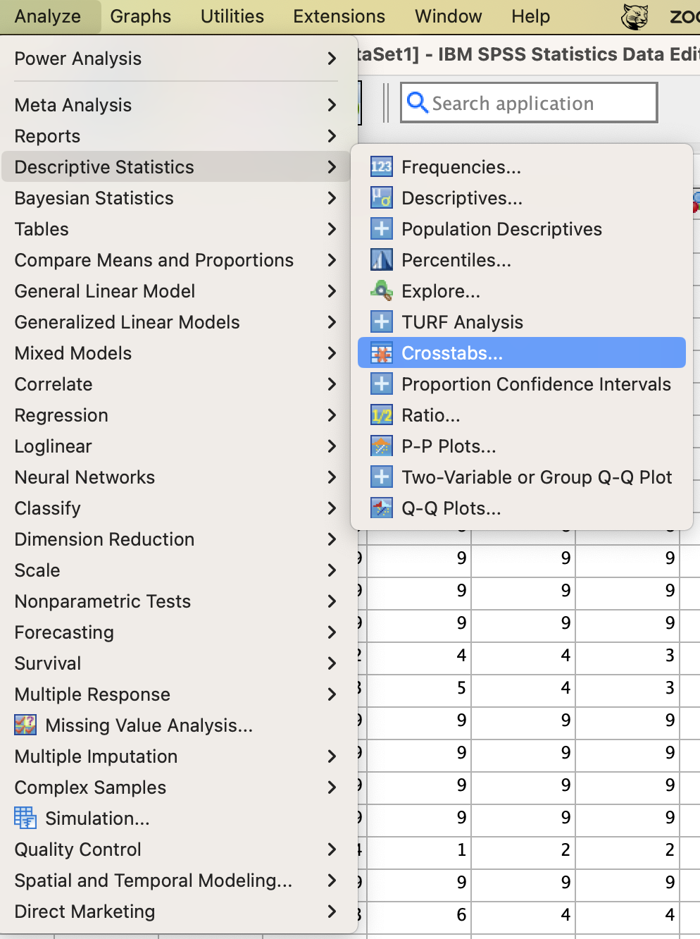
Menu:
First, go to Analyze → Descriptive Statistics → Crosstabs.
Next, put your independent variable into the "Column(s)" box and your dependent variable into the "Row(s)" box.
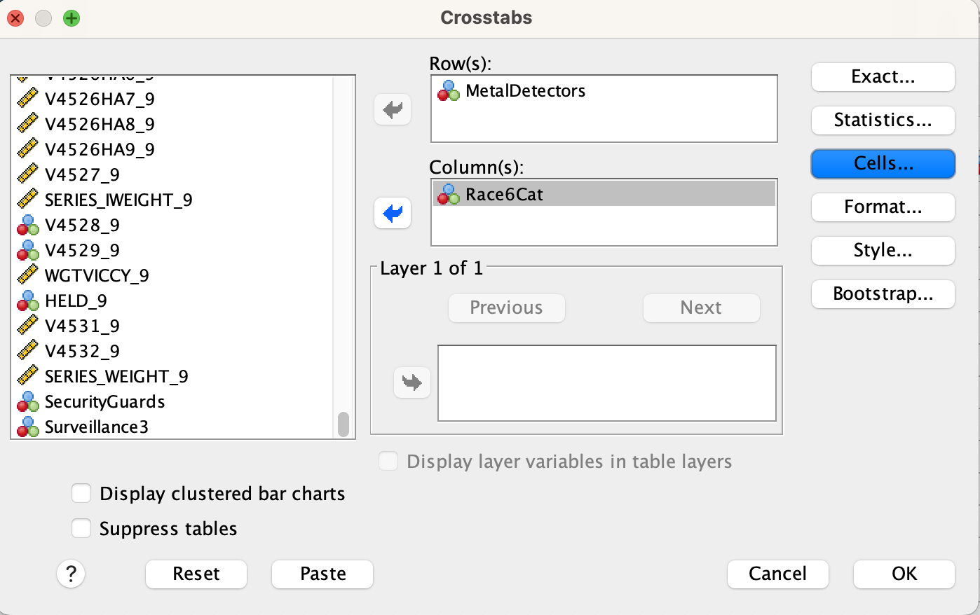
After that, click the "Cells" box on the right side. In the window that pops up, make sure that "Observed" is checked under "Counts." Under "Percentages," check the box for "Column." Don't check any other boxes. Click the "Continue" button.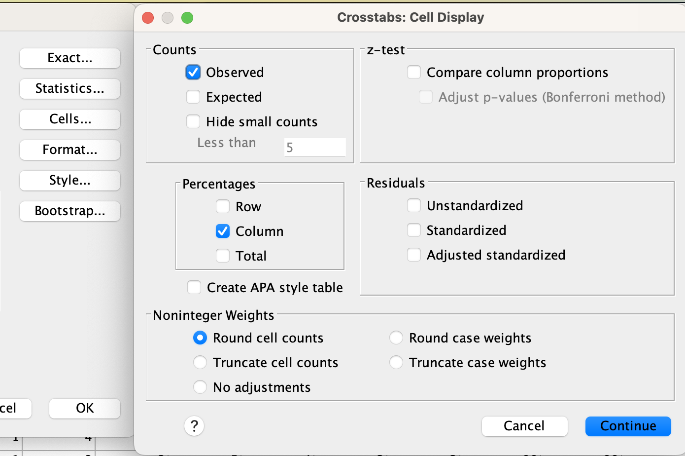
After that, go to the "Statistics" box on the right side. Check the box for "Chi-square" and click "Continue." 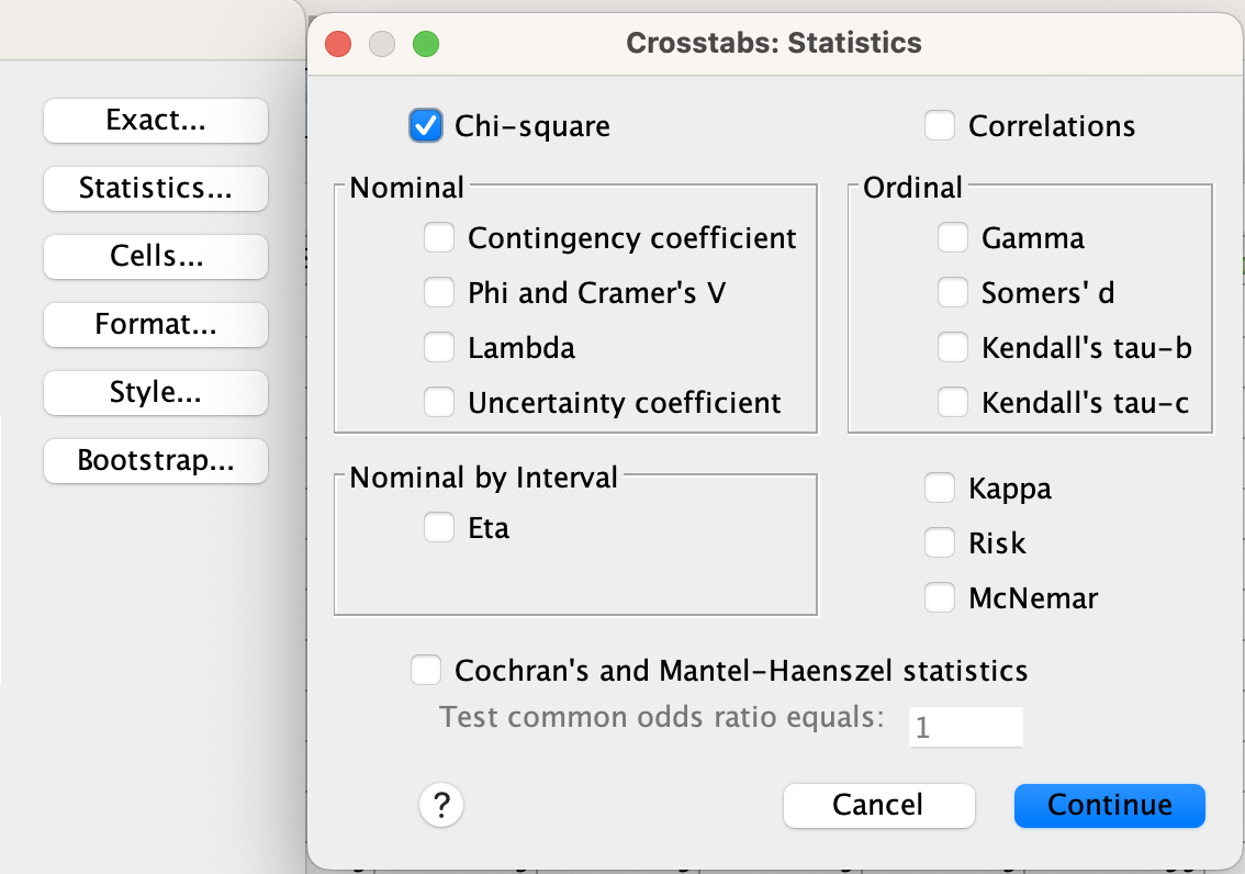
Finally, click "OK."
It's vital that your independent variable goes in the columns box and your dependent variable in the rows box, and not the other way around. Otherwise your column percentages will not match what you intend them to and you won't be able to make comparisons the same way.
Make sure to turn on column percentages. Without them, you can't make comparisons between categories given the differences in sample sizes among categories.
Don't check other boxes (like expected counts, or row percentages). These will add additional values to each cell that will be confusing.
Gamma
When you clicked in the "Statistics" box, another box you could check, under the "Ordinal" column, is "Gamma." Gamma is a descriptive statistic that measures strength and direction. It requires two ordinal-level variables, though sometimes indicator variables are used. Gamma ranges from -1 to +1. If the Gamma value is positive, that means that an increase in the independent variable is associated with an increase in the dependent variable. If the Gamma value is negative, that means that an increase in the independent variable is associated with a decrease in the dependent variable. The number measures strength by comparing positive to negative trends. A Gamma of zero indicates no relationship. The further away from zero, the stronger the relationship. Generally a Gamma value that is at least -0.3 or +0.3 indicates at least a moderate association, at least -0.5 or +0.5 indicates a substantial association, and at least -0.7 or +0.7 indicates a very strong association.
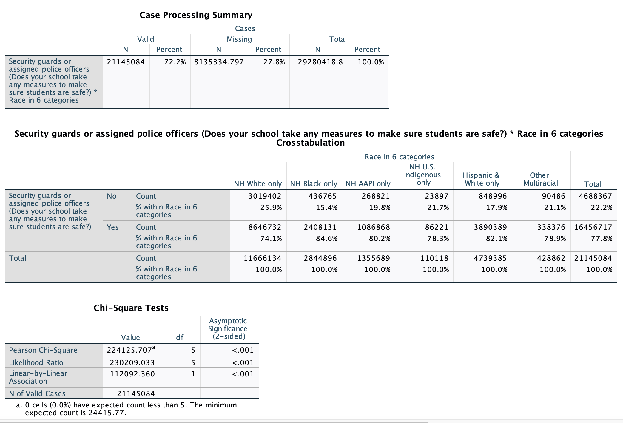
Here is our SPSS output for race and security guards:
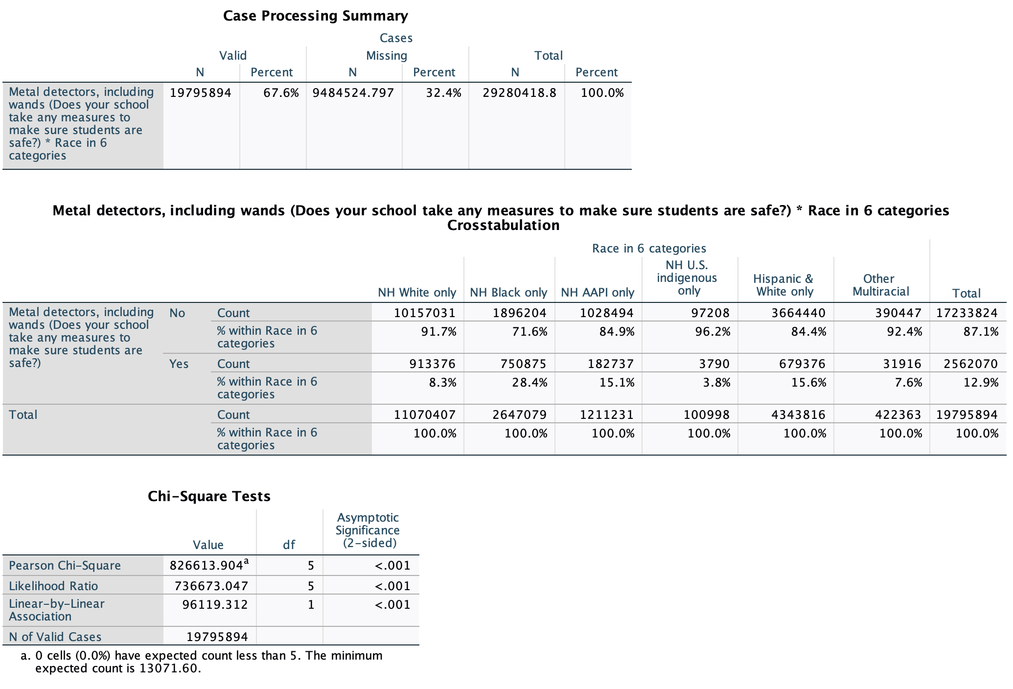
Here is our SPSS output for race and metal detectors:
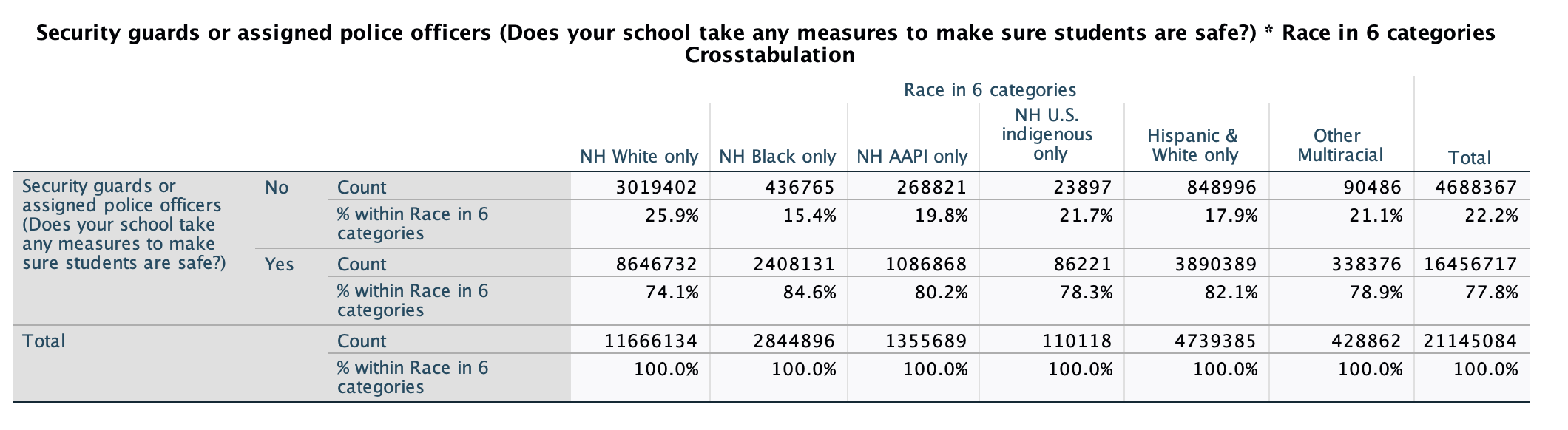
Looking at this crosstab, we can see six different races, as well as a total that includes everyone in the sample. For each racial category, it shows the distribution of whether respondents said they do or do not have a security guard or assigned police officer in their school. With the particular weighting used here, the frequencies are estimates of the target population. So for example, we would estimate that 3,019,402 non-Hispanic white only U.S. students ages 12 to 18 do not have a security guard or assigned police officer in their school (25.9% of respondents, just over 1/4), and that 8,646,732 U.S. students ages 12 to 18 do have a security guard or assigned police officer in their school (71.4% of respondents, just under 3/4).
How to look for and analyze relationships
The table's story includes answers to three questions:
- Is there a relationship?
- If so, how substantive it it?
- If so, what is the relationship? (E.g., what is its direction?)
1. Is there a relationship?
To analyze whether or not there is a relationship, look across rows and see if the percentages are the same or if they are different. Overall, 77.8% of student respondents report having security guards or police officers in their school. If there was no relationship between race and having security guards/police officers in one's school, then we would expect each racial category to have about 77.8% of student respondents reporting this. Look across and see what you notice.
Overall, 77.8% of students ages 12 to 18 are estimated to have a security guard or police officer in their school. That's over 3/4 of students. Each racial group also has somewhere between 74.1% and 84.6% of their respondents who reported having a security guard or police officer in their school. But don't make a common mistake of getting fooled into thinking there is no relationship just because most people have a security guard or police officer in their school, regardless of / across racial categories. We are trying to analyze variation. When I look across, I see that the percentage of students varies by race.
2. How substantive is the relationship?
Small percentage changes indicate a weak relationship. Substantial percentage changes indicate a strong relationship.
The biggest difference I see is that NH Black only respondents are over 10% more likely to report having a security guard or police officer in their school compared to NH White only respondents (84.6% vs. 74.1%). While what constitutes a substantive relationship is subjective, a good rule of thumb is to definitely characterize a relationship as being substantial anytime there is at least a 5% difference.
3. What is the relationship (e.g., what is its direction)?
If these were ordinal variables (e.g., age and income), we could classify the relationship by direction (e.g., as age increases, income increases). However, race is nominal so we cannot do that.
Looking at the crosstab, I am looking for which racial groups are more likely to have security guards or police officers in their school and which are less likely. I see that over 4/5 of NH Black only, Hispanic & White only, and NH AAPI only student respondents have security guards or assigned police officers in their school, between 3/4 and 4/5 of other multiracial and NH U.S. indigenous students do, and just under 3/4 of NH White only students do.
Try again with the crosstab below. Answer the three questions:
- Is there a relationship? (Do column percentages vary as you move across rows?)
- If so, how substantive it it? (Do they vary a lot?)
- If so, what is the relationship? (E.g., what is its direction?) (Which IV categories have higher and which have lower column percentages?)

Overall, just over 1/10 of student respondents report having metal detectors in their school (about 2.6 million children). When I compare the different column percentages for different racial groups, I see differences, with column percentages ranging from 3.8% to 28.4%. With a difference of over 25% between two of the racial groups, there appears to be a relationship, and it is a substantial one.
- 15.1% of NH AAPI only respondents and 15.6% of Hispanic & White only respondents reported having metal detectors in their schools. These are pretty similar. However, just because there is no substantive difference between two racial groups does not mean there is not an overall relationship between race and having metal detectors in one's school. It just means that the relationship only applies to differences between certain racial groups.
NH Black only students (respondents) are most likely to report having metal detectors in their school. Over 1/4 of these respondents reported this. Over 10% lower are Hispanic & White only and NH AAPI students, where over 1/7 of students reported this. Less than 1/10 of NH White only, other multiracial, and NH U.S. indigenous only students reported this. There are substantive differences. Indeed, while there are over 8 million more NH White only students ages 12-18 in the U.S. than NH Black students, only about 160,000 more NH White only students than NH Black only students are estimated to have metal detectors in their schools. NH Black students are over 20% more likely than NH White students to report having metal detectors in their schools. That's over 1 student out of every 5.
We know there is a relationship between race and whether or not a 12-16 year old U.S. student who took the School Crime Supplement survey has a police officer/security guard and/or a metal detector in their school. But we are not interested in those 14,273 respondents. The survey was conducted to allow us to generalize to all 12-16 year old U.S. students.
Chi-square (χ2) is an inferential statistic. It lets us evaluate population claims for categorical variables from representative data. If you have a cross-tab, chi-square is usually the corresponding statistical test you use for hypothesis testing.
Chi (χ) is a Greek letter. While it rhymes with chai, it starts with a k sound, not a ch sound. The inferential statistic is called chi-square (notated as χ2) because we square values when we are calculating it.
H∅: Null hypothesis
The null hypothesis is that there is no difference or no relationship (among your target population). In Chapter 7, the null hypothesis was also that there is no difference between the two variables in terms of their means, that they're equal. For chi-square, it's the same--- that the frequencies in our crosstab that we would expect if there was no relationship are equal to the frequencies we actually have from our sample.
Ha: Alternative hypothesis
The alternative hypothesis is that there is a relationship (among your target population). Chi-square tests to see whether the column percentages we were looking at before are different enough, taking into account sample size and the number of categories both variables have, such that we can claim they are likely different among our target population.
Significance and p-values:
From our chi-square test, we can use a chi-square table, or an online calculator like this one (for df, the degrees of freedom, use the total number of categories for both variables minus 2) to calculate our p-value. The more categories your variables have, the higher your chi-square value will need to be to pass the critical value corresponding to p=0.05. The p-value is the probability we would draw our random sample with the column percentages we did if there really was no relationship between the two variables.
For the p-value, look at the "Chi-Square Tests" output. The p-value is in the cell at the intersection of the "Pearson Chi-Square" row and the "Asymptomatic Significance (2-sided)" column.
Remember, our conventional standard is that if p<0.05, we reject our null, and claim there is a significant relationship. We are over 95% confident the two variables are related among our target population.
Security Guards/Police Officers
H∅: Null hypothesis There is no relationship among U.S. students ages 12-18 between race and whether or not there is a security guard or police officer assigned to a school.
Ha: Alternative hypothesis There is a relationship among U.S. students ages 12-18 between race and whether or not there is a security guard or police officer assigned to a school.
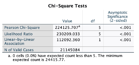
For the p-value, look at the cell at the intersection of the "Pearson Chi-Square" row and the "Asymptomatic Significance (2-sided)" column. Here, p<0.001. That is less than 0.05, so we reject our null hypothesis that there is no relationship. We are over 99.9% confident (1-0.001=99.9%) that there is a relationship, among all U.S. 12-18 year old students, between race and whether or not there is a security guard or police officer assigned to a school. (Note: Given the large sample size with weighting, I also ran chi-square with the unweighted data. The chi-square value was much lower, 52.3, but the p-value was still <0.001.)
Metal Detectors/Wands
H∅: Null hypothesis There is no relationship among U.S. students ages 12-18 between race and whether or not there are metal detectors, including wands, in the student's school.
Ha: Alternative hypothesis There is a relationship among U.S. students ages 12-18 between race and whether or not there are metal detectors, including wands, in the student's school.
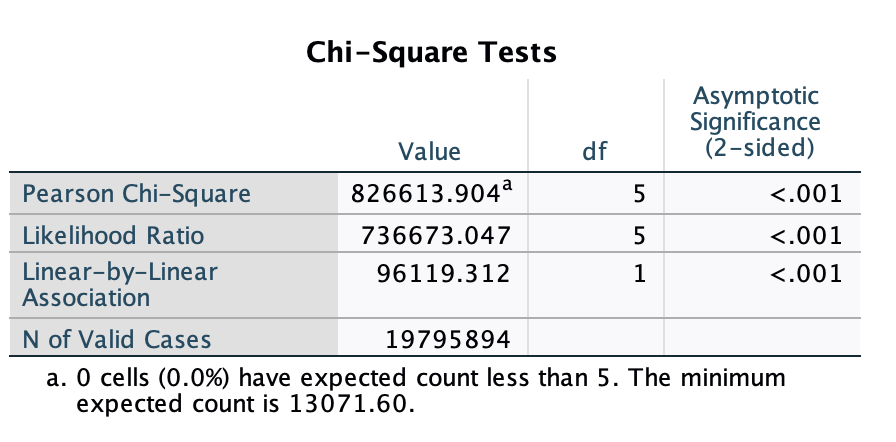
For the p-value, look at the cell at the intersection of the "Pearson Chi-Square" row and the "Asymptomatic Significance (2-sided)" column. Here, p<0.001. That is less than 0.05, so we reject our null hypothesis that there is no relationship. We are over 99.9% confident (1-0.001=99.9%) that there is a relationship, among all U.S. 12-18 year old students, between race and whether or not there are metal detectors, including wands, in the student's school. (Note: Given the large sample size with weighting, I also ran chi-square with the unweighted data. The chi-square value was much lower, 222.3, but the p-value was still <0.001.)
Among all students surveyed, 12.9% had metal detectors in their schools.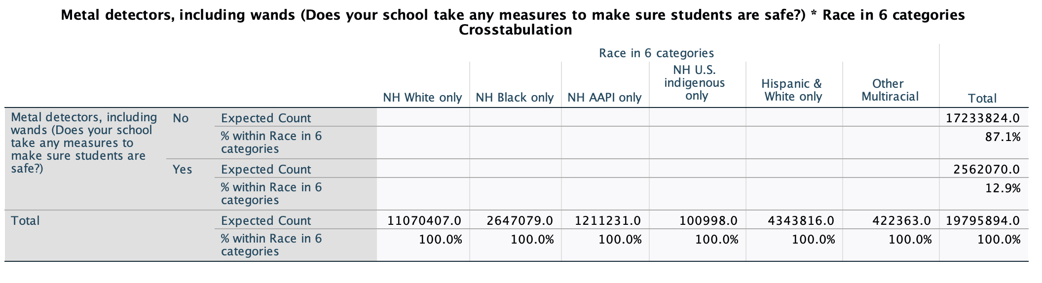
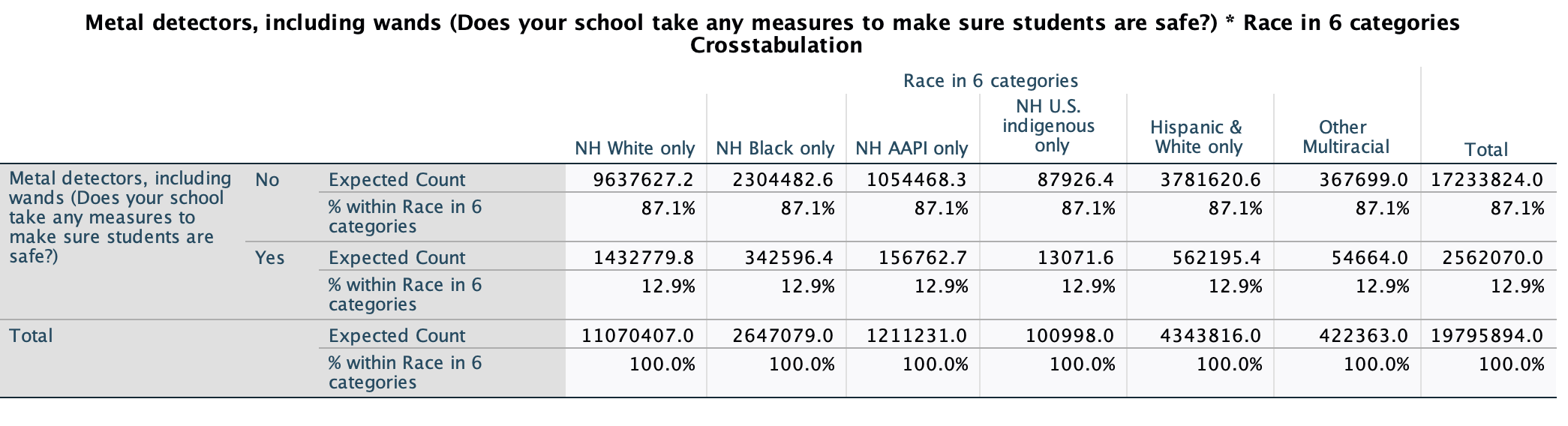
If there was no relationship between race and whether or not students have metal detectors in their schools, then we would expect that percentage to be the same across racial groups. 12.9% of NH White only students would have metal detectors in their schools, 12.9% of NH Black only students would have metal detectors in their schools, 12.9% of NH AAPI only students, etc.
We would end up with an expected crosstab that looks like this:
Instead, our actual sample, our observed crosstab, looks like this:
Our null hypothesis is that the observed and expected frequencies are equal, that these two tables match.
For each cell, we use the formula: (fo-fe)2÷fe where f is for frequency, o is for observed, and e is for expected. For example, for NH White only students saying "no" to having metal detectors, the expected frequency (if there was no relationship, if 87.1% of NH White only respondents had said no) is 9,637,627.2. The observed frequency, the actual number who said "no" (weighted) was 91.7% of the sample, 10,157,031.
(fo-fe)2÷fe=(10,157,031-9,637,627.2)2 ÷ 9,637,627.2=27,992.4
I would then do this for each of the other cells (NH White only Yes, NH Black only No, NH Black only yes, etc.). Then I would find the sum of these numbers. The bigger the differences between the actual data and expected data, the bigger the chi-square value. The bigger the chi-square value, the smaller the p-value.