
9: Elaborated Crosstabs
- Page ID
- 189328

\( \newcommand{\vecs}[1]{\overset { \scriptstyle \rightharpoonup} {\mathbf{#1}} } \)
\( \newcommand{\vecd}[1]{\overset{-\!-\!\rightharpoonup}{\vphantom{a}\smash {#1}}} \)
\( \newcommand{\dsum}{\displaystyle\sum\limits} \)
\( \newcommand{\dint}{\displaystyle\int\limits} \)
\( \newcommand{\dlim}{\displaystyle\lim\limits} \)
\( \newcommand{\id}{\mathrm{id}}\) \( \newcommand{\Span}{\mathrm{span}}\)
( \newcommand{\kernel}{\mathrm{null}\,}\) \( \newcommand{\range}{\mathrm{range}\,}\)
\( \newcommand{\RealPart}{\mathrm{Re}}\) \( \newcommand{\ImaginaryPart}{\mathrm{Im}}\)
\( \newcommand{\Argument}{\mathrm{Arg}}\) \( \newcommand{\norm}[1]{\| #1 \|}\)
\( \newcommand{\inner}[2]{\langle #1, #2 \rangle}\)
\( \newcommand{\Span}{\mathrm{span}}\)
\( \newcommand{\id}{\mathrm{id}}\)
\( \newcommand{\Span}{\mathrm{span}}\)
\( \newcommand{\kernel}{\mathrm{null}\,}\)
\( \newcommand{\range}{\mathrm{range}\,}\)
\( \newcommand{\RealPart}{\mathrm{Re}}\)
\( \newcommand{\ImaginaryPart}{\mathrm{Im}}\)
\( \newcommand{\Argument}{\mathrm{Arg}}\)
\( \newcommand{\norm}[1]{\| #1 \|}\)
\( \newcommand{\inner}[2]{\langle #1, #2 \rangle}\)
\( \newcommand{\Span}{\mathrm{span}}\) \( \newcommand{\AA}{\unicode[.8,0]{x212B}}\)
\( \newcommand{\vectorA}[1]{\vec{#1}} % arrow\)
\( \newcommand{\vectorAt}[1]{\vec{\text{#1}}} % arrow\)
\( \newcommand{\vectorB}[1]{\overset { \scriptstyle \rightharpoonup} {\mathbf{#1}} } \)
\( \newcommand{\vectorC}[1]{\textbf{#1}} \)
\( \newcommand{\vectorD}[1]{\overrightarrow{#1}} \)
\( \newcommand{\vectorDt}[1]{\overrightarrow{\text{#1}}} \)
\( \newcommand{\vectE}[1]{\overset{-\!-\!\rightharpoonup}{\vphantom{a}\smash{\mathbf {#1}}}} \)
\( \newcommand{\vecs}[1]{\overset { \scriptstyle \rightharpoonup} {\mathbf{#1}} } \)
\(\newcommand{\longvect}{\overrightarrow}\)
\( \newcommand{\vecd}[1]{\overset{-\!-\!\rightharpoonup}{\vphantom{a}\smash {#1}}} \)
\(\newcommand{\avec}{\mathbf a}\) \(\newcommand{\bvec}{\mathbf b}\) \(\newcommand{\cvec}{\mathbf c}\) \(\newcommand{\dvec}{\mathbf d}\) \(\newcommand{\dtil}{\widetilde{\mathbf d}}\) \(\newcommand{\evec}{\mathbf e}\) \(\newcommand{\fvec}{\mathbf f}\) \(\newcommand{\nvec}{\mathbf n}\) \(\newcommand{\pvec}{\mathbf p}\) \(\newcommand{\qvec}{\mathbf q}\) \(\newcommand{\svec}{\mathbf s}\) \(\newcommand{\tvec}{\mathbf t}\) \(\newcommand{\uvec}{\mathbf u}\) \(\newcommand{\vvec}{\mathbf v}\) \(\newcommand{\wvec}{\mathbf w}\) \(\newcommand{\xvec}{\mathbf x}\) \(\newcommand{\yvec}{\mathbf y}\) \(\newcommand{\zvec}{\mathbf z}\) \(\newcommand{\rvec}{\mathbf r}\) \(\newcommand{\mvec}{\mathbf m}\) \(\newcommand{\zerovec}{\mathbf 0}\) \(\newcommand{\onevec}{\mathbf 1}\) \(\newcommand{\real}{\mathbb R}\) \(\newcommand{\twovec}[2]{\left[\begin{array}{r}#1 \\ #2 \end{array}\right]}\) \(\newcommand{\ctwovec}[2]{\left[\begin{array}{c}#1 \\ #2 \end{array}\right]}\) \(\newcommand{\threevec}[3]{\left[\begin{array}{r}#1 \\ #2 \\ #3 \end{array}\right]}\) \(\newcommand{\cthreevec}[3]{\left[\begin{array}{c}#1 \\ #2 \\ #3 \end{array}\right]}\) \(\newcommand{\fourvec}[4]{\left[\begin{array}{r}#1 \\ #2 \\ #3 \\ #4 \end{array}\right]}\) \(\newcommand{\cfourvec}[4]{\left[\begin{array}{c}#1 \\ #2 \\ #3 \\ #4 \end{array}\right]}\) \(\newcommand{\fivevec}[5]{\left[\begin{array}{r}#1 \\ #2 \\ #3 \\ #4 \\ #5 \\ \end{array}\right]}\) \(\newcommand{\cfivevec}[5]{\left[\begin{array}{c}#1 \\ #2 \\ #3 \\ #4 \\ #5 \\ \end{array}\right]}\) \(\newcommand{\mattwo}[4]{\left[\begin{array}{rr}#1 \amp #2 \\ #3 \amp #4 \\ \end{array}\right]}\) \(\newcommand{\laspan}[1]{\text{Span}\{#1\}}\) \(\newcommand{\bcal}{\cal B}\) \(\newcommand{\ccal}{\cal C}\) \(\newcommand{\scal}{\cal S}\) \(\newcommand{\wcal}{\cal W}\) \(\newcommand{\ecal}{\cal E}\) \(\newcommand{\coords}[2]{\left\{#1\right\}_{#2}}\) \(\newcommand{\gray}[1]{\color{gray}{#1}}\) \(\newcommand{\lgray}[1]{\color{lightgray}{#1}}\) \(\newcommand{\rank}{\operatorname{rank}}\) \(\newcommand{\row}{\text{Row}}\) \(\newcommand{\col}{\text{Col}}\) \(\renewcommand{\row}{\text{Row}}\) \(\newcommand{\nul}{\text{Nul}}\) \(\newcommand{\var}{\text{Var}}\) \(\newcommand{\corr}{\text{corr}}\) \(\newcommand{\len}[1]{\left|#1\right|}\) \(\newcommand{\bbar}{\overline{\bvec}}\) \(\newcommand{\bhat}{\widehat{\bvec}}\) \(\newcommand{\bperp}{\bvec^\perp}\) \(\newcommand{\xhat}{\widehat{\xvec}}\) \(\newcommand{\vhat}{\widehat{\vvec}}\) \(\newcommand{\uhat}{\widehat{\uvec}}\) \(\newcommand{\what}{\widehat{\wvec}}\) \(\newcommand{\Sighat}{\widehat{\Sigma}}\) \(\newcommand{\lt}{<}\) \(\newcommand{\gt}{>}\) \(\newcommand{\amp}{&}\) \(\definecolor{fillinmathshade}{gray}{0.9}\)Chapter 9 introduces multivariate analysis. We will build on Chapter 8's focus on crosstabs and chi-square by breaking down our crosstabs by a third variable.
In Chapter 8, we found that, in the United States, as of 2019, non-Hispanic black students were much more likely than non-Hispanic white students to have metal detectors (including wands) in their schools.
Is this a causal relationship? Many U.S.-Americans think we live in a post-racial society where racism no longer exists. Let's say someone claims that the relationship is actually spurious --- that social class is a preceding variable that explains away the relationship. Let's put aside how racism contributes towards a higher proportion of black students being lower-income than white students. We can test whether the black-white metal detector gap is simply due to income differences, or whether race is a contributing factor. The way we do this is to control for income. We will hold income constant in order to isolate the effect of race on having a metal detector in school from the effect of income on having a metal detector in school.
Control variable: An additional variable added to a model and held constant in order to improve our evaluation of relationships with the dependent variable.
- For our bivariate (two variable) crosstab, we asked, "Is there a relationship between a student's race and whether or not they have metal detectors in their school?"
- When we add a control variable, we add a second question, "Does this relationship differ by [the control variable]?". In this case, does the relationship differ by social class?
Chapter 8 involved bivariate statistics, because we were using two variables. Here in Chapter 9, we are adding a third variable, the control variable, so we are now engaging in multivariate statistics, because we are using multiple, more than two, variables.
When we control for income using crosstabs, we generate a series of partial crosstabs of the same race-metal detector relationship. We can evaluate whether the relationship exists and what it looks like among lower-income students, among middle-income students, and among higher-income students. If income explains away the race-metal detector relationship, once we control for income, there should not be a relationship between race and having metal detectors in one's school in any of the partial crosstabs. So for example, holding income constant, if race is not a factor, low-income students should have the same rates of metal detectors in their schools regardless of race / across racial groups.
Partial crosstabs, also called elaborated crosstabs, are crosstabulations that add a control variable to the original bivariate crosstab, producing separate bivariate crosstabs for each subgroup.
Here we will make a series of crosstabs among income subgroups.
Total: Race (NH black vs. NH white) & Metal Detectors in Schools
First, let's look at our bivariate crosstab and chi-square again. Sometimes you will see a smaller sample size when you look at the overall bivariate crosstab using an elaborated/partial crosstab, because cases are only included if there is useful data for all three variables. In this case, we have income data for all 3,942 students that we had race and metal detector data on, so the sample size is the same.
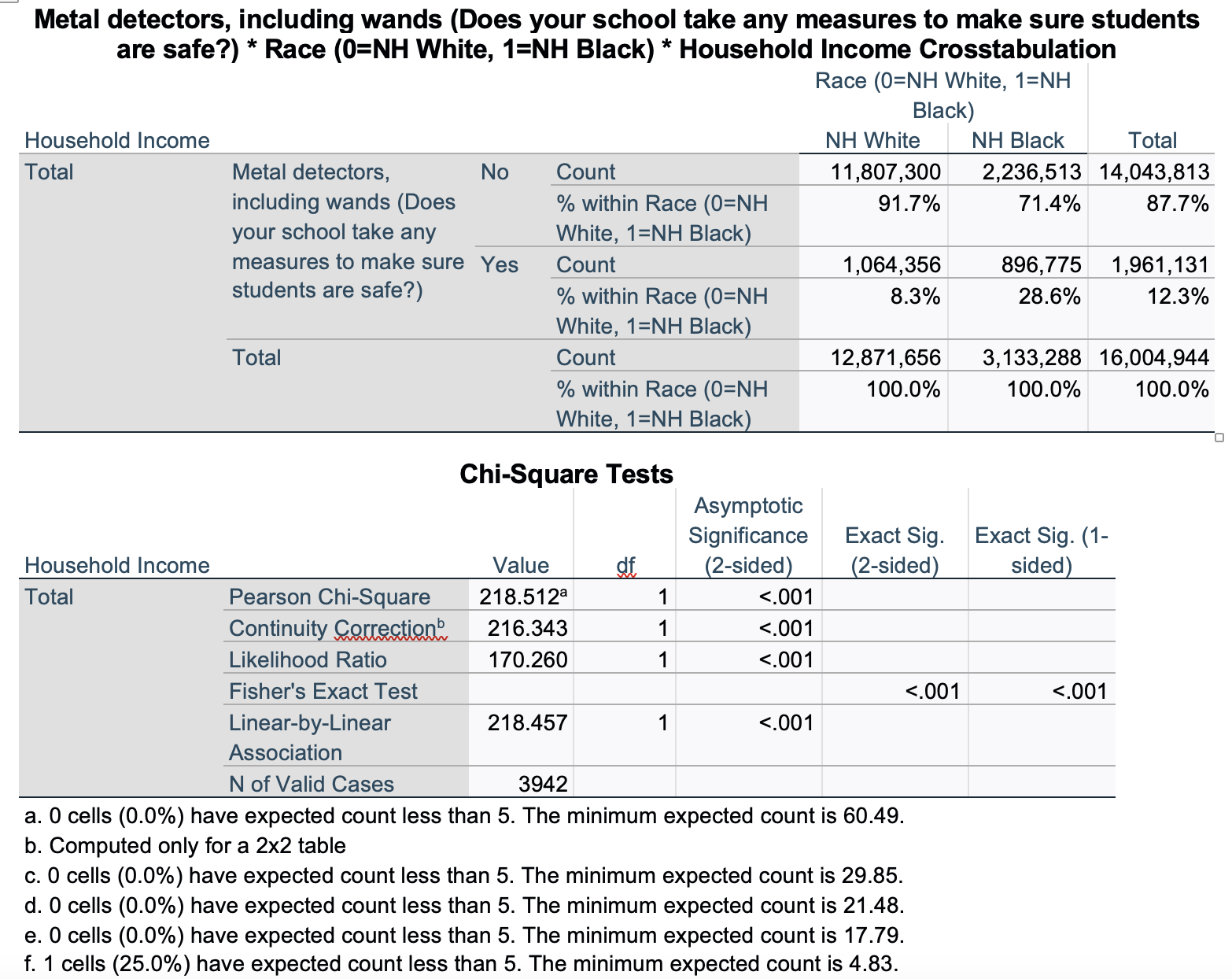
I am over 99.9% confident there is a relationship among all U.S. students 12 to 18 years old between being NH black vs. NH white and having metal detectors in schools. In the sample, NH black students are over 20% more likely to have metal detectors in their schools compared to NH white students.
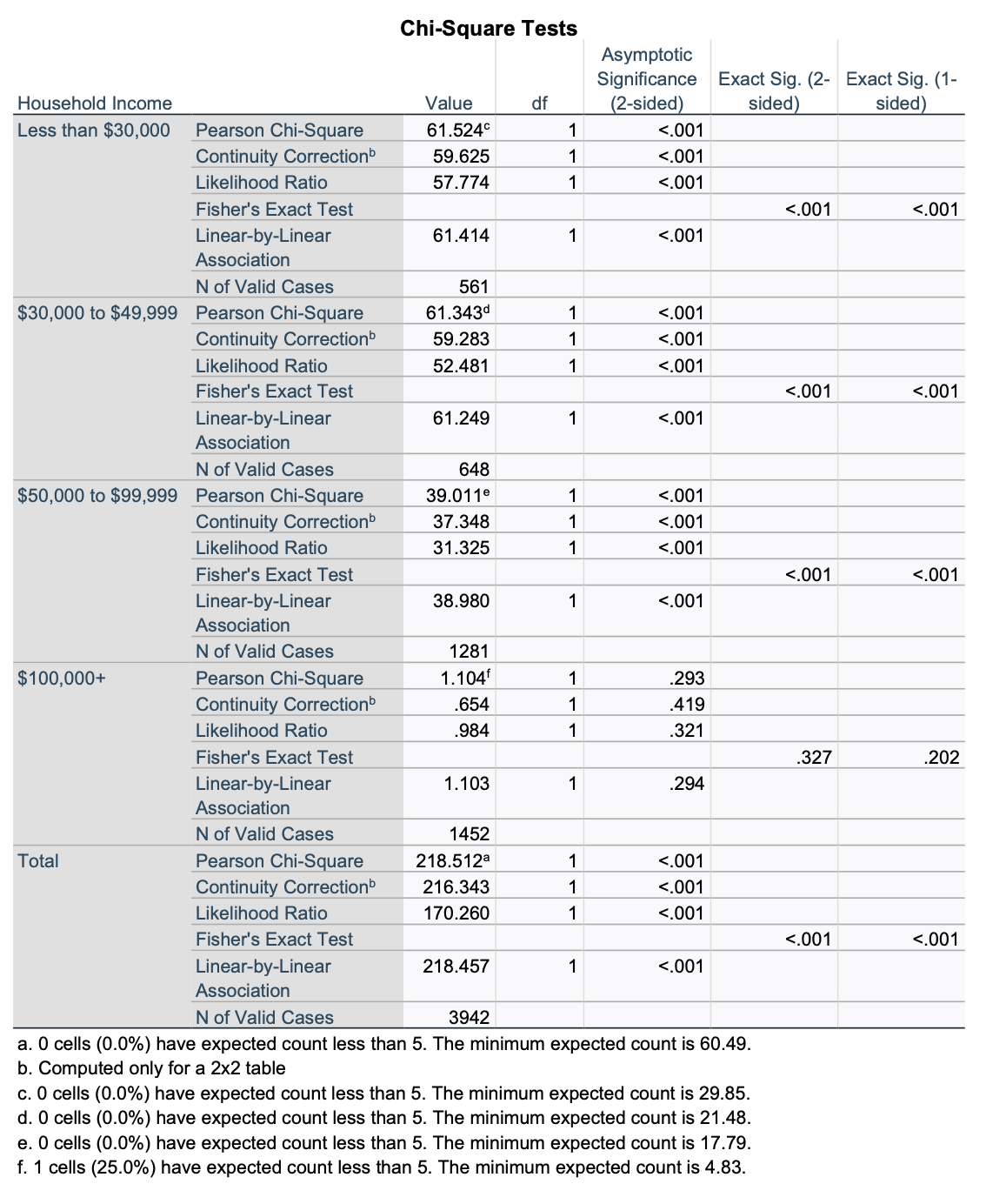
Because of the large sample size generated from weighting (since it calculated estimates of all 12 to 18 year old students, over 16 million cases), almost all chi-square tests are going to give me significant results (here it was p<0.001, and this continues for all the ones below). Instead, for the chi-square test above (and the ones I show below) I ran chi-square with weighting off to reflect the actual number of respondents.
Household Income <$30,000: Race (NH black vs. NH white) & Metal Detectors in Schools
Now let's look at the same relationship, but just among students whose household income is less than $30,000.
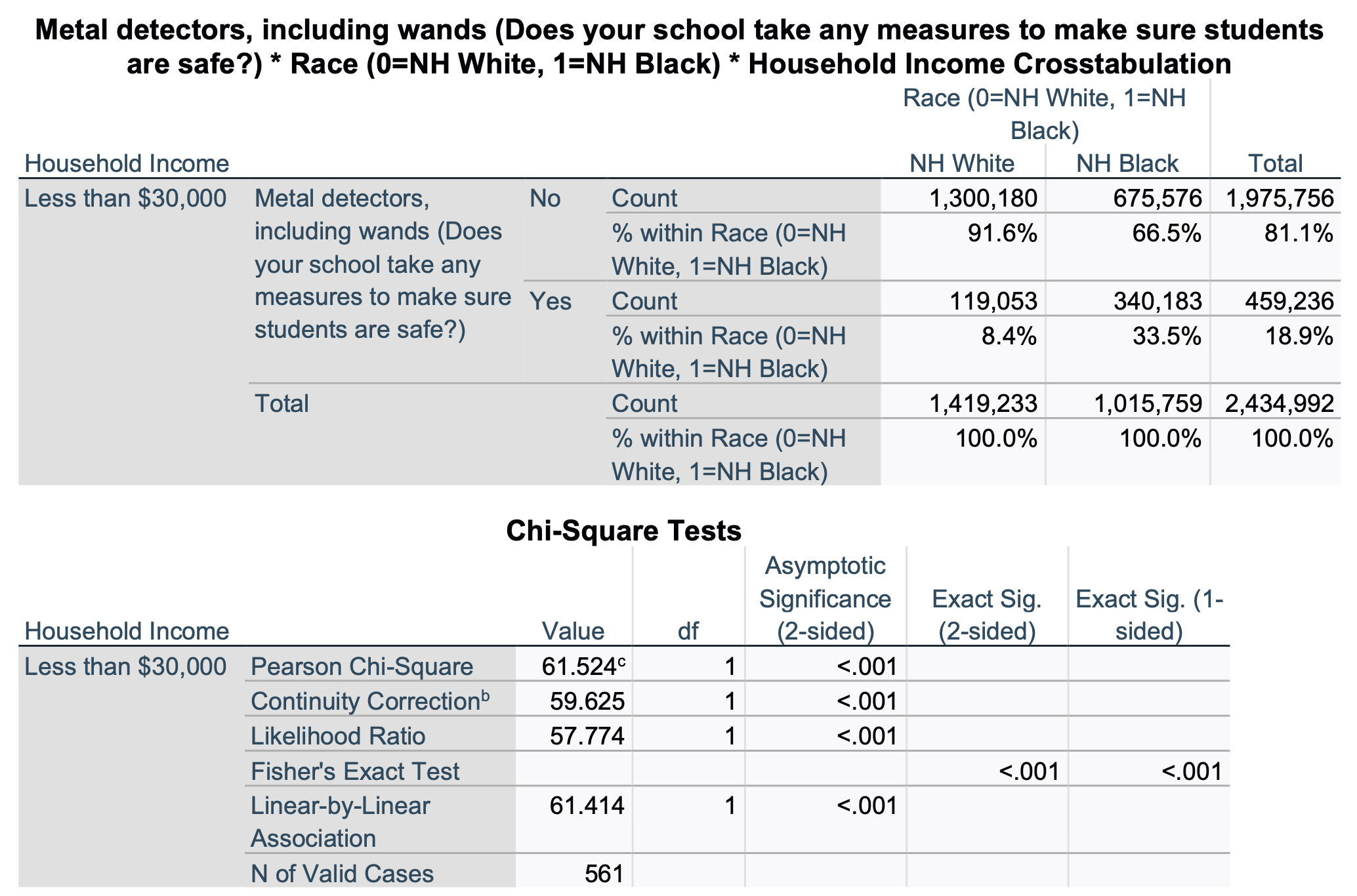
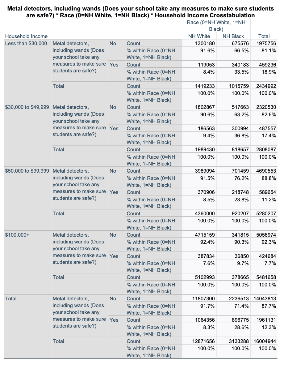
For this partial crosstab, our target population is not all U.S. students 12-18 years old. It is a subset of this population: all U.S. students 12-18 years old who have household incomes less than $30,000. We are over 99.9% confident that, among U.S. students 12-18 years old who have household incomes less than $30,000, there is a relationship between being NH white vs. black and whether or not one has metal detectors in their school. In the sample, NH black students (from households with incomes <$30K) are over 25% more likely than NH white students (from households with incomes <$30K) to have metal detectors in their schools. We now know that the race gap for metal detectors in schools is not simply a matter of income. Among lower income households, there is still a race gap between NH white and NH black students. In fact, it got wider, not smaller.
We can also compare our first and second crosstab, and observe that, compared to all students in the sample, NH white students from households with less than $30,000 have about the same likelihood of having metal detectors in their school (8.4% vs 8.3%). However, in the sample 7% more poor NH black students have metal detectors in their schools compared to NH black students as a whole (33.5% vs. 28.6%). The race gap actually got wider when we looked at poor students. It didn't go away.
Household Income $30,000 to $49,999: Race (NH black vs. NH white) & Metal Detectors in Schools
Now let's look at the same relationship, but just among students whose household income is at least $30K but less than $50K.
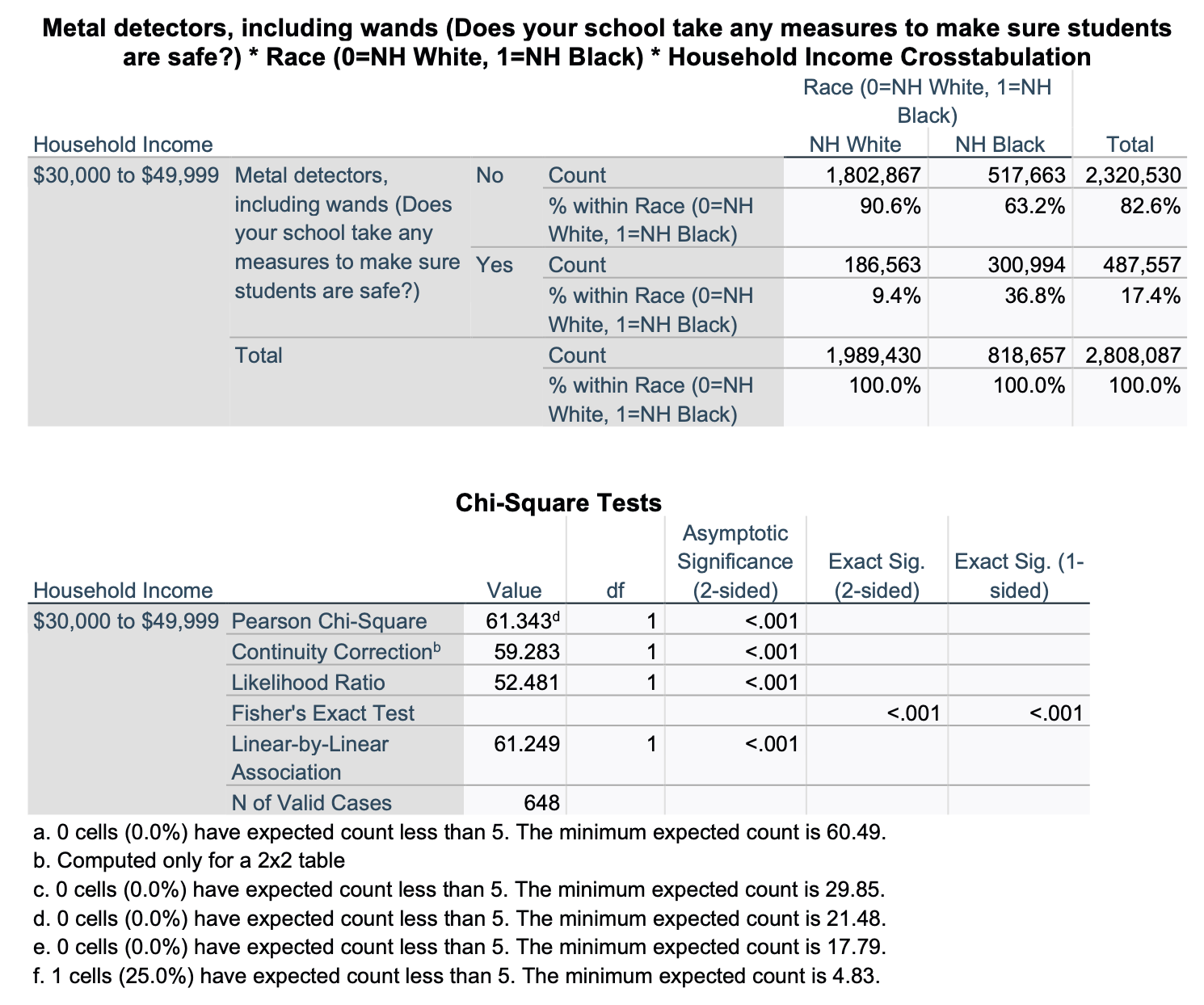
For this partial crosstab, our target population is not all U.S. students 12-18 years old. It is a subset of this population: all U.S. students 12-18 years old who have household incomes in the $30Ks and $40Ks. We are over 99.9% confident that, among U.S. students 12-18 years old who have household incomes between $30,000 and $49,999, there is a relationship between being NH white vs. black and whether or not one has metal detectors in their school. In the sample, NH black students (from households with incomes $30K to <$50K) are over 25% more likely than NH white students (from households with incomes $30K to <$50K) to have metal detectors in their schools. We again find here the race gap for metal detectors in schools is not simply a matter of income. Among households making between $30,000 and $49,999, there is still a race gap between NH white and NH black students.
Household Income $50,000 to $99,999: Race (NH black vs. NH white) & Metal Detectors in Schools
Now let's look at the same relationship, but just among students whose household income is at least $50K but less than $100K.
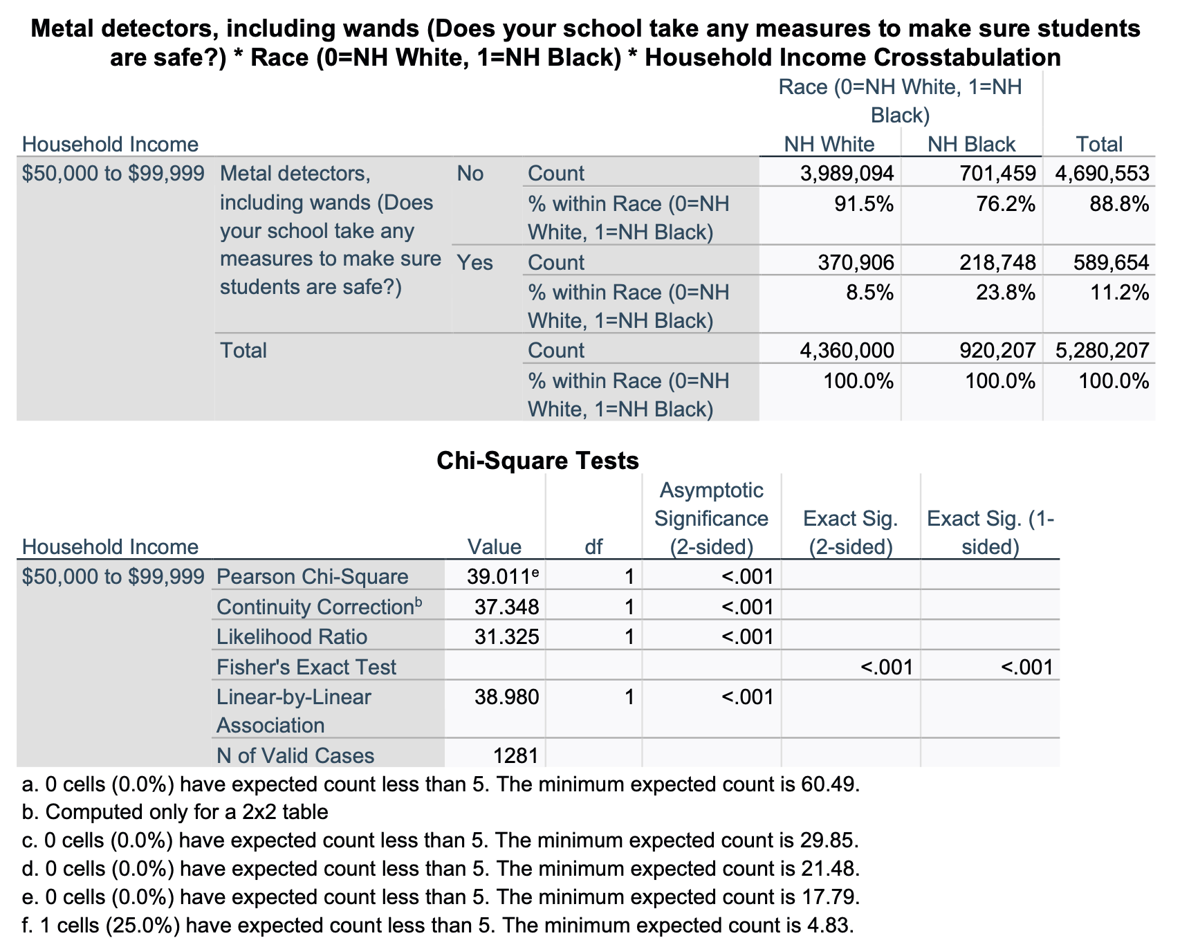
For this partial crosstab, our target population is not all U.S. students 12-18 years old. It is a subset of this population: all U.S. students 12-18 years old who have household incomes between $50,000 and $99,999. We are over 99.9% confident that, among U.S. students 12-18 years old who have household incomes between $50,000 and $99,999, there is a relationship between being NH white vs. black and whether or not one has metal detectors in their school. In the sample, NH black students (from households with incomes $50K to <$100K) are over 15% more likely than NH white students (from households with incomes $50K to <$100K) to have metal detectors in their schools. We again find here the race gap for metal detectors in schools is not simply a matter of income. Among households making between $50,000 and $99,999, there is still a race gap between NH white and NH black students.
Household Income $100,000+: Race (NH black vs. NH white) & Metal Detectors in Schools
Now let's look at the same relationship, but just among students whose household income is at least $100K.
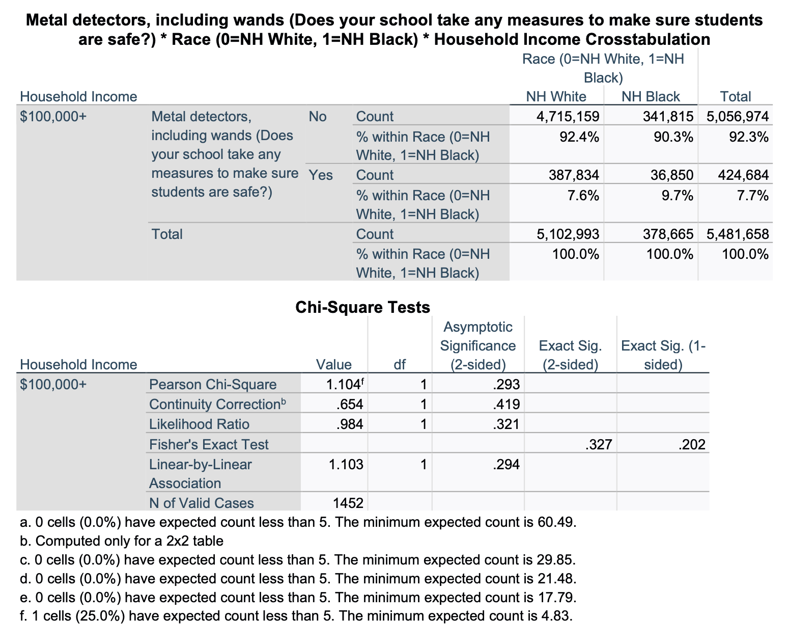
For this partial crosstab, our target population is not all U.S. students 12-18 years old. It is a subset of this population: all U.S. students 12-18 years old who have household incomes $100,000 or higher. Our p-value (unweighted) is p=0.293. We are not over 95% confident that, among U.S. students 12-18 years old who have household incomes $100,000 or higher, there is a relationship between being NH white vs. black and whether or not one has metal detectors in their school. We could be making a Type 2 error (false negative), as there are only 73 NH black students in our sample who have household incomes $100,000 or higher (1,379 NH white students). However, we cannot claim, based on this data, that there is a NH black-NH white race gap among students from households making $100,000 or higher. In the sample, NH black students (from households with incomes $100K+) are just over 2% more likely than NH white students (from households with incomes $100K+) to have metal detectors in their schools.
Putting It Together
Income did not make the relationship between race and having a metal detector spurious. It did, however, moderate it. Overall in our sample, about 1 in 5 (20.3%) more NH black students had metal detectors in their schools compared to NH white students. However, for those from households with incomes less than $30,000 or $30,000 to $49,999, this was about 1 in 20 students higher (about 25%), for students from $50,000 to $99,999, about 1 in 20 students fewer (about 15%), and among students $100,000, the sample difference was about 1 in 50 (2.1%) students, and we were not confident that there is any difference for this subgroup. It may be that wealthy students, regardless of race, are less likely to have metal detectors in their schools, but that among lower-income and middle-income students, there is a sizeable race gap.
Elaborated Crosstab:
- IV: Race (NH black vs. NH white)
- DV: Metal Detectors in Schools
- Control Variable: Household income
The SPSS outputs above started with an overall crosstab between the IV and DV and then showed partial crosstabs, with the same IV and DV but broken down among subsamples based on household income. When you run an elaborated crosstab in SPSS, all this information comes out in one table, all together.
Here are the series of crosstabs, for each income group and then the "total."
Here are the chi-square outputs. SPSS runs a separate chi-square test for each of the (five above) crosstabs.
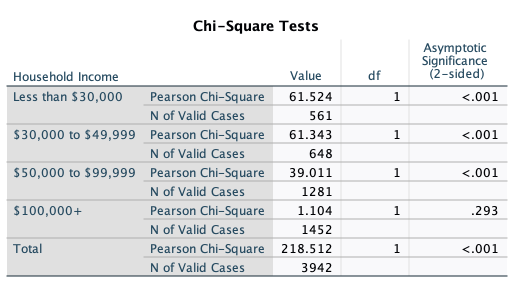
Given the length of the chi-square outputs, you may want to delete extra information so it is easier to look at and make comparisons. Remember that in SPSS you can double-click on outputs and then highlight and delete rows, columns, etc., that you do not want to appear. Here is a simplified version of the chi-square output, where I can focus on the p-values for each chi-square test.
Follow the same process you did in Chapter 8, with one additional step (highlighted in yellow below).
Syntax:
CROSSTABS
/TABLES=DependentVariableName BY IndependentVariableName BY ControlVariableName
/FORMAT=AVALUE TABLES
/STATISTICS=CHISQ
/CELLS=COUNT COLUMN
/COUNT ROUND CELL.
Menu:
First, go to Analyze → Descriptive Statistics → Crosstabs.
Next, put your independent variable into the "Column(s)" box, your dependent variable into the "Row(s)" box, and your control variable into the "Layer 1 of 1" box.

After that, click the "Cells" box on the right side. In the window that pops up, make sure that "Observed" is checked under "Counts." Under "Percentages," check the box for "Column." Don't check any other boxes. Click the "Continue" button.
After that, go to the "Statistics" box on the right side. Check the box for "Chi-square" and click "Continue."
Finally, click "OK."
In the example above, we added a control variable, analyzed our initial bivariate crosstab and chi-square test, our partial crosstabs and chi-square tests, and then compared the bivariate model to the multivariate model. From this we figured out what happened to our original relationship after we added the control variable.
While you can analyze what happens when you add a control variable this way, there is a more systematic way to do so.
When you add a control variable, there are five potential outcomes:
- the initial relationship stays the same
- the initial relationship goes away
- the initial relationship diminishes
- the initial relationship varies
- the initial relationship increases (or there was no relationship, and now a relationship appears)
Interpreting the effects of adding a control variable can further depend on whether the control variable is an antecedent variable or intervening variable.
Antecedent variables are variables that precede, that come before, both the independent and dependent variables.
Antecedent → Independent → Dependent
Example: Degree → Occupation → Salary
Intervening variables are variables that come in between the independent and dependent variables.
Independent → Intervening → Dependent
Example: Going to a restaurant → Eating → Satiety
Let's take a made-up example with made-up data of a bivariate relationship between finding a four-leaf clover and winning raffles. In our bivariate model, people who found a 4-leaf clover in the past year were also more likely to win a raffle in the past year.
We'll consider two different control variables.
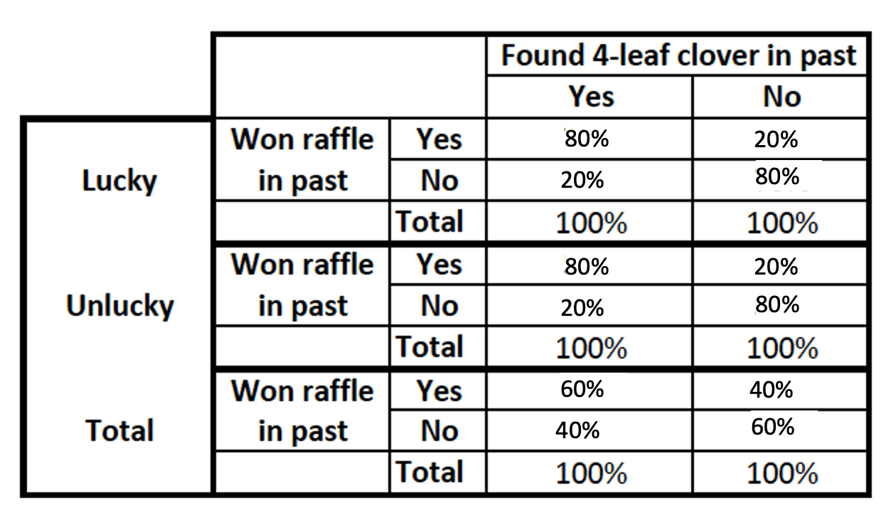
- The first is an antecedent variable, luck. Maybe lucky people are more likely to find 4-leaf clovers and win the raffle, and unlucky people are less likely to do either?
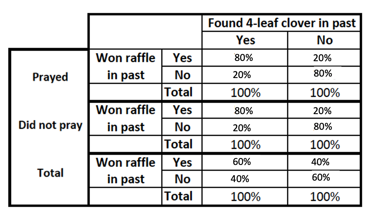
- The second is an intervening variable, praying to win a raffle. Maybe people who find a 4-leaf clover decide to put their luck to use, pray to win a raffle, and through doing so end up more likely to win a raffle.
The relationship stays the same → Replication
If the bivariate relationship stays the same, then the relationship still exists, even after controlling for the additional variable.
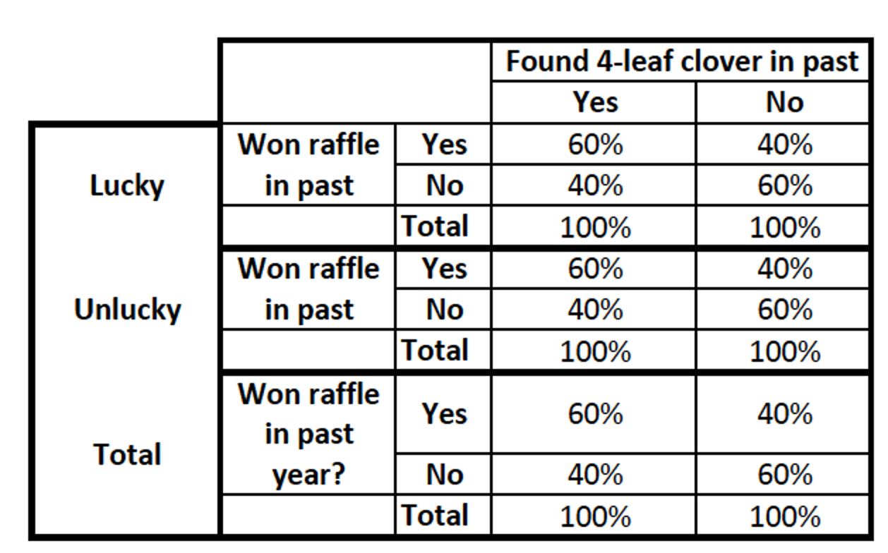
There was no change after controlling for luck. Luck does not explain the relationship.

There was no change after controlling for praying. Praying does not affect the relationship.
The relationship goes away
- Antecedent = Spurious
With an antecedent variable, if the bivariate relationship goes away, then the relationship is explained by the control (also called confounding) variable.
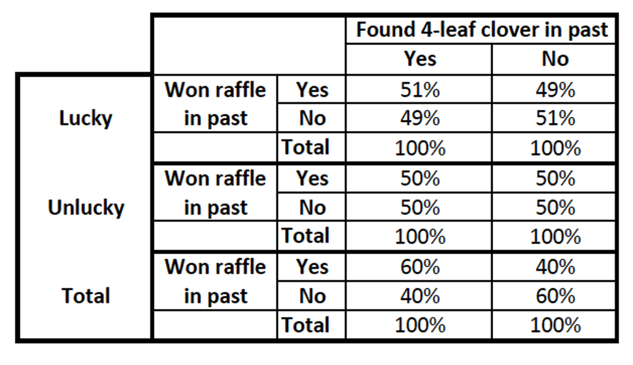
The relationship went away. The relationship between finding a 4-leaf clover and winning a raffle is spurious. Luck explains the relationship.
- Intervening = Mediation
If the bivariate relationship goes away, then the relationship's mechanism is explained by the control variable.
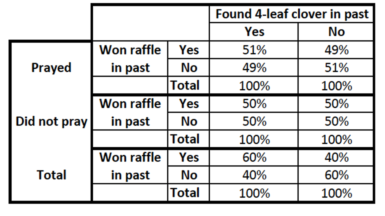
The relationship went away. Praying mediates (explains) the relationship. Praying is the mechanism through which finding a 4-leaf clover turns into winning a raffle. People who find 4 leaf clovers then pray to win raffles and then (perhaps enter more raffles and then) win raffles. The relationship is not spurious, because praying did not come before finding the 4-leaf clover.
The relationship decreases → Partially explained
In these examples, the relationship still exists, but it is less substantive than it was prior to introducing the control variable. In these cases, the control variable partially explains the relationships.
Antecedent:

The relationship is not as substantive. The relationship is partially explained by the control variable, but the IV still has its own independent effect. Luck partially explains the relationship.
Intervening:

The relationship is not as substantive. The way that finding a four-leaf clover translates into winning a raffle is partially explained by praying, but there are other mechanisms at play as well.
The relationship varies → Moderation
If the bivariate relationship varies / is different among subgroups, then the relationship is moderated by the control variable, meaning the control variable affects the relationship. For different control variable values, the relationship may be smaller, larger, etc.
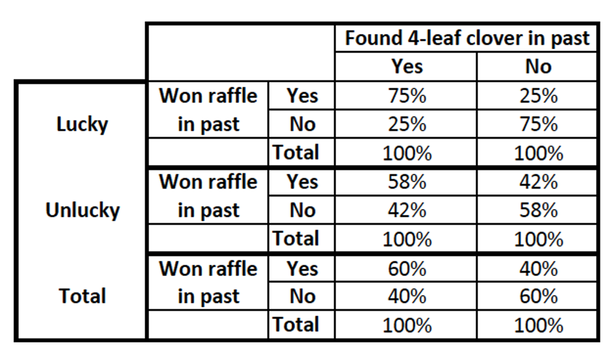
The relationship changes depending on whether someone is lucky or not. Luck moderates the relationship. The relationship looks different for folks who are lucky (where finding a 4 leaf clover is even more substantially associated with winning a raffle) and folks who are not lucky (finding a 4-leaf clover helps, but not at all as much).
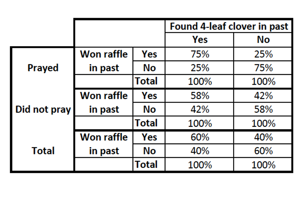
The relationship changes depending on whether someone prays to win a raffle or not. Praying moderates the relationship. The relationship looks different for folks who do and do not pray to win.
Relationship increases or appears
- Relationship increases
The effect of the finding clovers increased when controlling for luck, because luck un-supresses some of the power of finding a four leaf clover. Finding a clover especially makes a difference among people who are lucky, and also among people who are unlucky. After controlling, the relationship grows stronger/larger.
The effect of the finding clovers increasing when controlling, because prayer un-supresses some of the power of finding a four leaf clover. Finding a clover especially makes a difference among people who prayed, and also among people who did not pray. After controlling, the relationship grows stronger/larger.
- Relationship appears
What if we had initially found no relationship between finding a 4-leaf clover and winning a raffle? Then, after adding our control variable, the relationship appeared?

The effect of the finding clovers was concealed, but controlling for luck revealed its effect, un-supressing the underlying pattern. The relationship has emerged, in context. Finding a 4-leaf clover makes a difference among those who are lucky and among those who are not lucky.

The effect of the finding clovers was concealed, but controlling for prayer revealed its effect/un-supressed the underlying pattern. The relationship has emerged, in context. Finding a 4-leaf clover makes a difference among those who pray and among those who don‘t.
Suppression effects do actually happen. For example, when I was analyzing support for public/employer sourcing of childcare funding using the 2012 General Social Survey, in my initial bivariate analysis, there was not a significant relationship between gender and support for public or employer sourcing of childcare funding. However, once I controlled for family income and political ideology, there was a relationship --- and men were more supportive! This relationship between gender and support for public or employer sourcing of childcare funding existed --- among the control variable groups. For example, if you hold family income and political ideology constant, say liberals with low family incomes, you'll find men are slightly more supportive. However, when I looked at the bivariate relationship, this is not what I found. That's because women tend to be more liberal and less conservative, and tend to have lower family incomes. So when I'm comparing gender among all U.S. adults, women's decreased support that I found after controlling for the other variables was balanced out by there being more women who are liberal and low-income who have increased support. Here income and political ideology are suppressor variables.
- The initial relationship stays the same
- Replication: relationship still exists
- The initial relationship goes away
- If control variable is antecedent
- Spurious: Relationship explained by control (confounding) variable
- If control variable is intervening
- Relationship's mechanism explained by control (mediating) variable
- If control variable is antecedent
- The initial relationship diminishes
- If control variable is antecedent
- Relationship is partially explained by control variable, but original independent variable still has its own independent effect
- If control variable is intervening
- Relationship's mechanism is partially but not fully explained by control variable
- If control variable is antecedent
- The initial relationship varies
- Moderation: relationship differs/interacts with control variable
- The initial relationship increases (or there was no relationship, and now a relationship appears)
- Suppression: Relationship was suppressed, relationship is explained by its effect within control variable groups
Let's take a look at one final example. This example comes from the ANES survey following the 2020 election, where eligible voters were asked how they felt about Black Lives Matter, using a feelings thermometer ranging from 0 to 100:
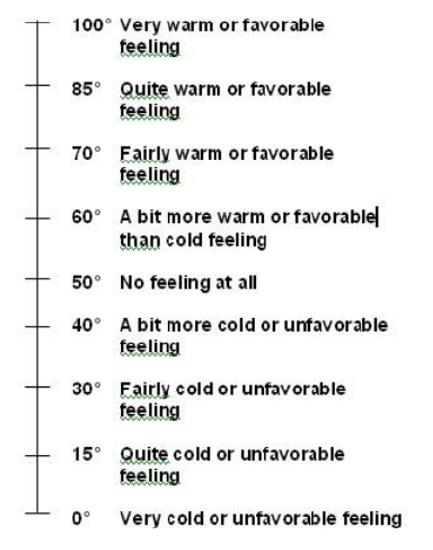
I collapsed the feelings thermometer into 5 categories: 0° (coldest), 1° to 49° (cold), 50° (neutral), 51° to 99° (warm), and 100° (warmest).
My independent variable is political ideology, measures as conservative, moderate, or liberal. Presumably the more liberal one is, the more likely one will be supportive of Black Lives Matter. However, I am going to add a control variable from a survey question that asks, "How much discrimination have you personally faced because of your ethnicity or race?" To what extent will people's personal experiences of racism impact their views on Black Lives Matter, regardless of their political ideology?
Here is the SPSS output:
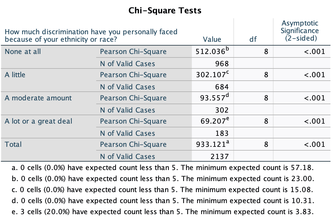
From the chi-square test, we can see that we are over 99.9% confident there is a relationship between political ideology and feelings towards BLM among U.S. eligible voters. We can see that this relationship also holds among subgroups of U.S. eligible voters who have experienced different levels of racism. For example, even among those who have experienced "a lot or a great deal" of racism, we are confident there is a relationship between political ideology and feelings towards BLM.
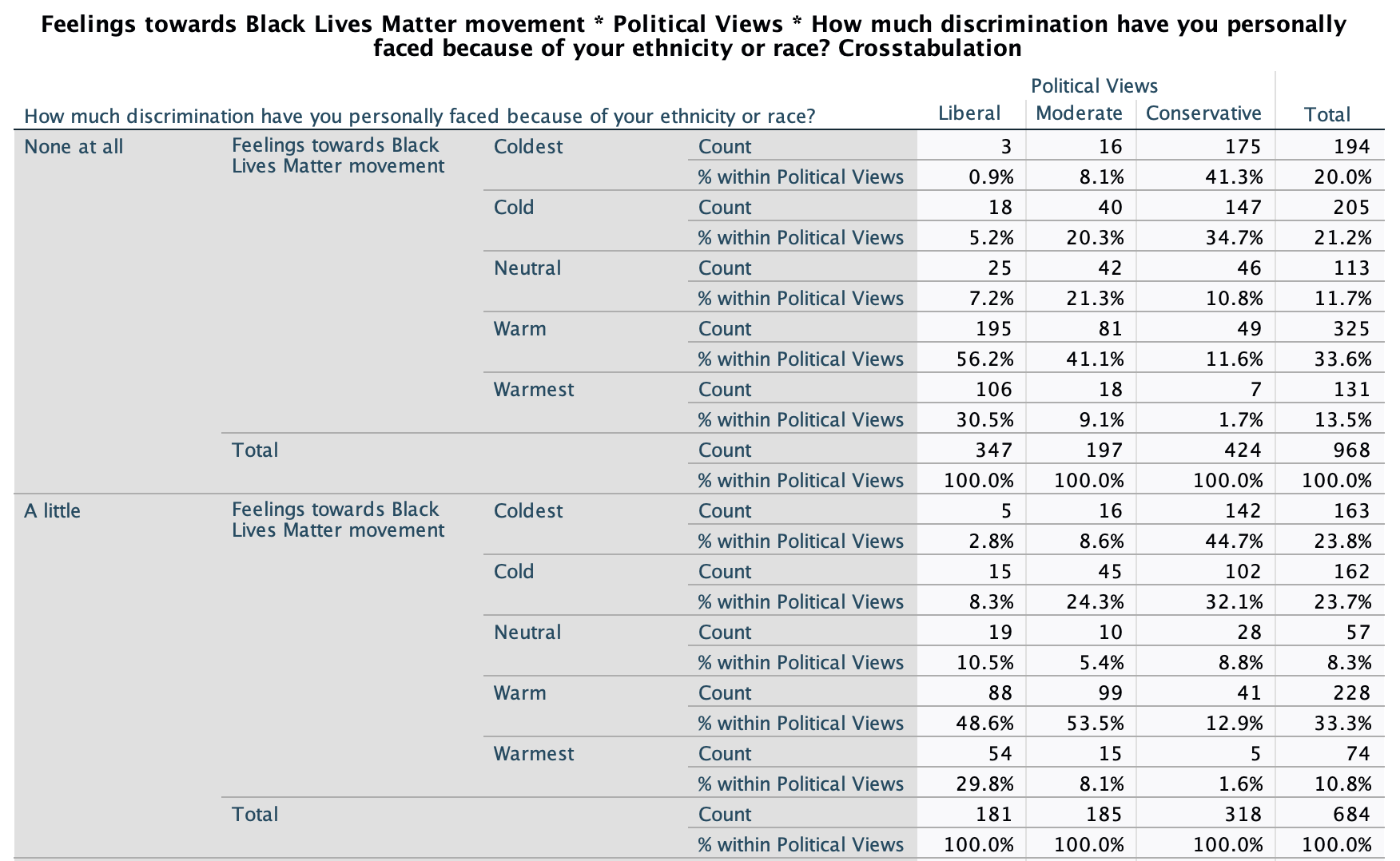
Turning to the crosstab, let's examine the actual relationship and what story the table tells us. It's always a good idea to start with the "Total" section of the table at the bottom to get a sense of the bivariate relationship.
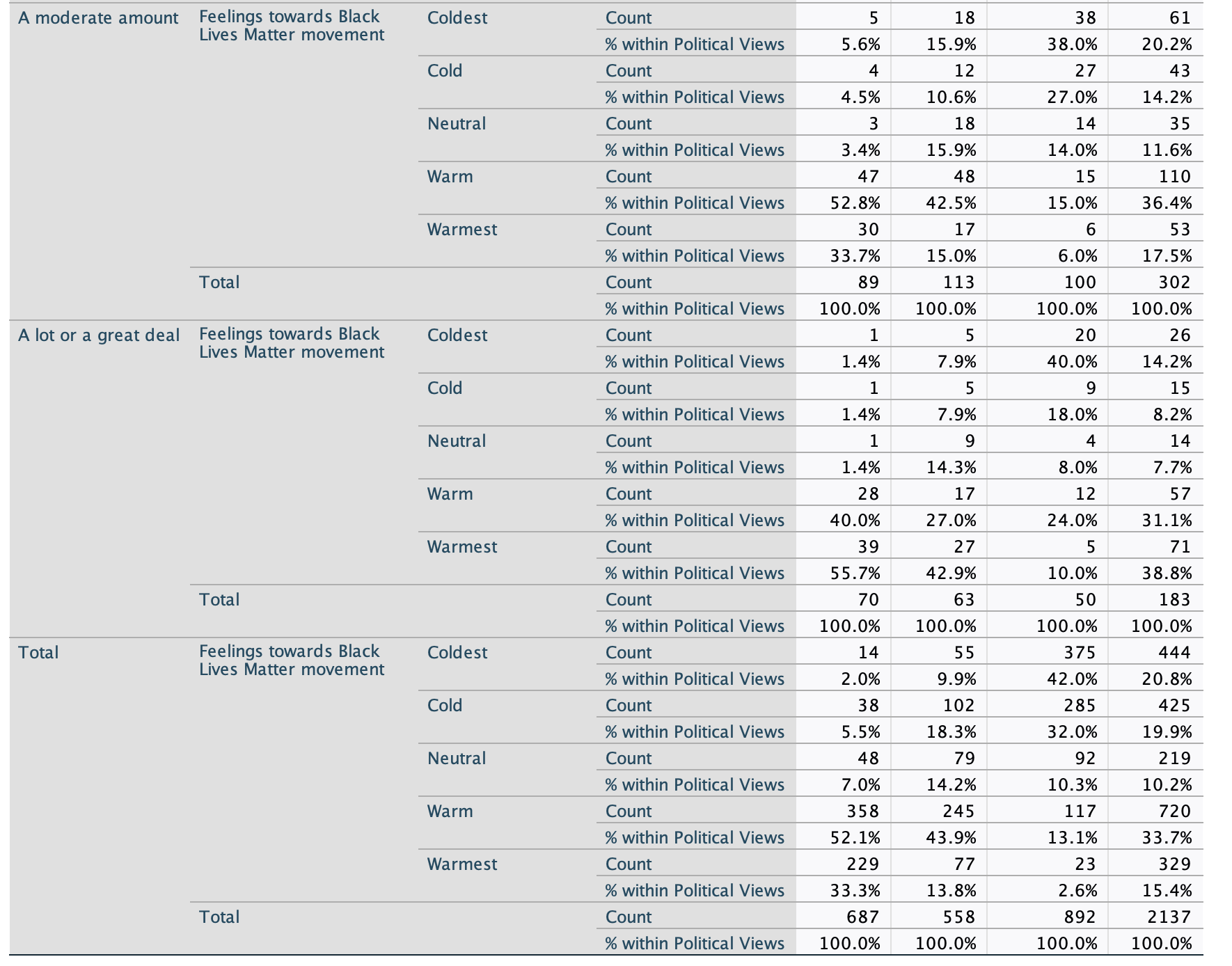
As expected, generally the more liberal one is the warmer their feelings towards BLM. We can see that while 2.6% of conservatives have the warmest (100 degree) feelings towards BLM, this increases to 13.8% for moderates and 33.3% for liberals. Conversely, while 2.0% of liberals have the coldest (0 degree) feelings towards BLM, this increases to 9.9% for moderates and 33.3% for liberals.
Looking at all the partial crosstabs, these directions hold out among all subgroups of eligible voters with different levels of experiences of racism. However, there are some differences.
Let's zoom in on the column percentages for those who have the coldest and the warmest feelings:
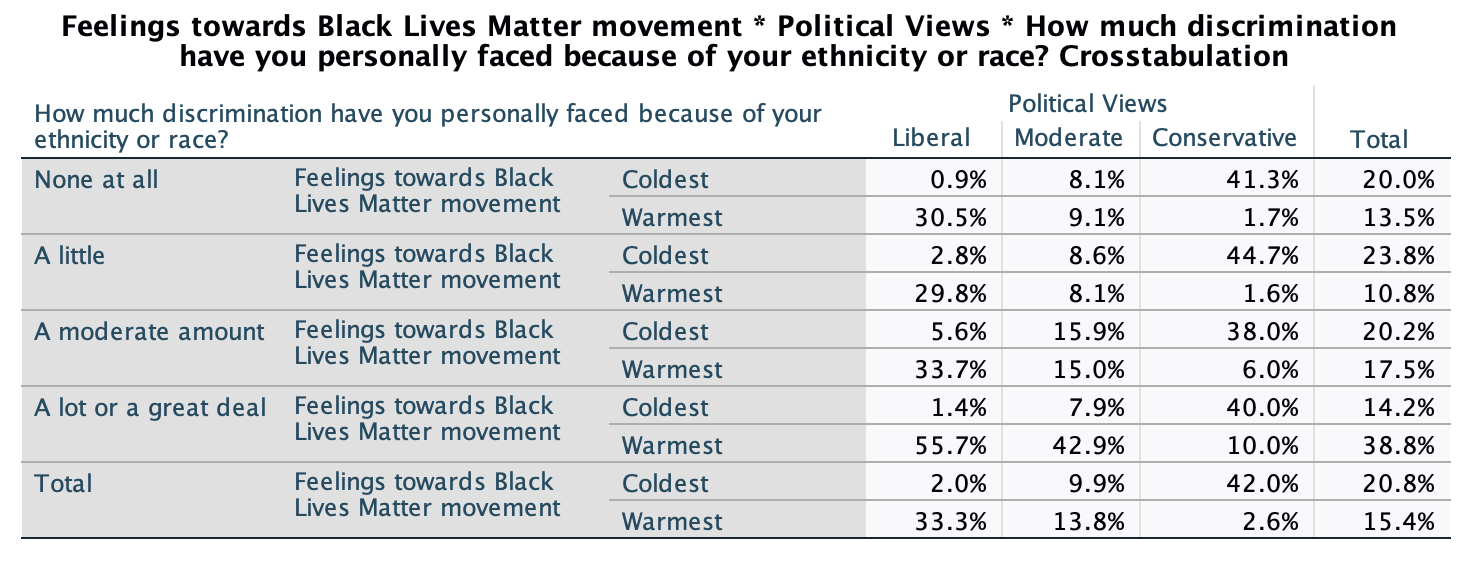
Those who have not experienced any racism are pretty similar to those who have experienced a little racism. Liberals don't have much change once we get to a moderate amount of racism, but there's a jump among moderates both in having the coldest and the warmest feelings towards BLM, and while only at 6%, the percentage of conservatives with the warmest feelings towards BLM more than triples. Finally, for those who have experienced a lot or a great deal of racism, we see a substantial increase among liberals and among moderates in having the warmest feelings (for liberals from close to 1/3 to a majority, for moderates from 8.1% to 15.0% to 42.9%). Conservatives see their highest proportion having the warmest feelings towards conservatives (1/10), though across levels of experiences of racism, about 2/5 of conservatives still have the coldest feelings towards BLM.