Up to this point, our emphasis has been on the output decisions of firms. A primary goal has been to establish that firms’ output decisions respond to market price as predicted by the law of supply. However, when firms choose output, they must choose inputs. Input choices are also important to profit maximization. Let us briefly consider the problem of simultaneously choosing an output level and the necessary inputs to achieve it. To do so, it will first be necessary to introduce the idea of a production function. A production function is a mathematical representation of the production technology by which inputs are converted into an output. To keep things simple, consider a production technology with two inputs, \(x_{1}\) and \(x_{2}\) that can be converted into an output, \(q\).
\(q = f(x_{1}, x_{2})\)
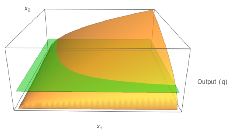
Figure \(\PageIndex{1}\) presents a three-dimensional rendering of a production function. Output increases as either of the inputs increases. However, it is common in economics to assume that production functions are concave. This is a mathematical way of saying that production functions exhibit the law of diminishing marginal productivity that was described earlier in the chapter. The example production function in Figure \(\PageIndex{1}\) is concave in that output increases at higher levels of inputs \(x_{1}\) and/or \(x_{2}\) but at a decreasing rate. The production surface shown in Figure \(\PageIndex{1}\) always slopes upward (moving away from the origin) but becomes less steep as increasing amounts of either of the inputs are employed.
Figure \(\PageIndex{1}\): Three-dimensional rendering of a production function. The production function is shown in yellow/orange tones. The green, horizontal plane intersects the production function at a fixed level of output. The origin is at the bottom left of the diagram.
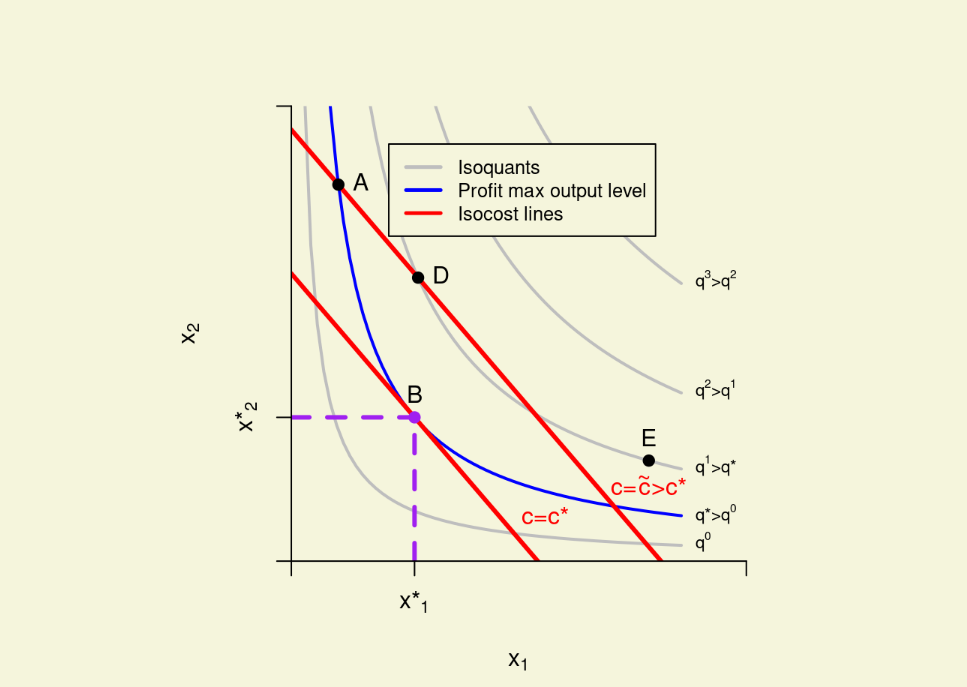
Because three dimensions is often hard to work with, a production function is typically rendered in two dimensions using an isoquant map similar to that shown below in Figure \(\PageIndex{2}\). To help you visualize the connection between the three-dimensional rendering in Figure \(\PageIndex{1}\) and the two dimensional rendering in Figure \(\PageIndex{2}\), consider the green plane that intersects the production function in Figure \(\PageIndex{1}\) above. The points where this plane intersects the function represent different combinations of \(x_{1}\) and \(x_{2}\) that could be used to obtain a fixed level of output equal to the elevation of the plane. If you were to look at this intersection directly from above, you would see an isoquant similar to one of the grey curves in Figure \(\PageIndex{2}\) below. In Figure \(\PageIndex{2}\), any point on the same isoquant represents a feasible way to produce a fixed level of output from the two inputs. Different isoquants could be obtained from Figure \(\PageIndex{1}\) by raising or lowering the horizontal plane to correspond to a different levels of output. The word, isoquant, is a combination of the prefix “iso”, meaning equal, and the word “quantity”. Thus, you can think of isoquants as “equal quantity curves”. For example, Points D and E in Figure \(\PageIndex{2}\) would each produce the same output level. Point D uses more of the \(x_{2}\) input and less of the \(x_{1}\) input than does point E. Nevertheless, each point represents a production plan that will achieve the same level of output. Using a conventional geographic orientation to Figure \(\PageIndex{2}\), it can be seen that isoquants in a northeasterly direction indicate higher levels of output.
Figure \(\PageIndex{2}\): Two dimensional rendering of the production function with the profit maximizing production plan depicted by point B. Superscripts are used to indicate different levels of output and are not exponents.
Figure \(\PageIndex{2}\) also shows isocost lines. Again as the name implies, an isocost line plots out production plans that cost the same. Production cost can be expressed in terms of inputs as follows:
\(c = W_{1}x_{2}\)
where \(W_{1}\) and \(W_{2}\) are the prices of inputs 1 and 2, respectively. Solving this expression algebraically for \(x_{2}\) provides the isocost lines depicted in Figure \(\PageIndex{2}\). These are of the form
Two isocost lines are depicted in Figure \(\PageIndex{2}\). One maps out all plans that provide a cost level of \(c = c*\). To the northeast of this is another isocost line that maps out all plans providing a higher cost level of \(c = \tilde{c})\). In Figure \(\PageIndex{2}\), the production plans represented by points A and D both cost \(c = \tilde{c} )\) because they are each on the isocost line even though more output is produced at D than at A (D lies on an isoquant that is northeast of A).
With these preliminaries, Figure \(\PageIndex{2}\) can be used to visualize the firm’s profit maximization problem. Suppose that at the prevailing output and input prices, the firm’s profit maximizing choice is to set its output at \(q = q*\). This is represented by the blue isoquant in Figure \(\PageIndex{2}\). The firm must choose a production plan that produces \(q*\) at the lowest cost possible. The profit maximizing production plan is represented by point B in Figure \(\PageIndex{2}\). To see why point B is the profit maximizing production plan, consider an alternative production plan like point A. This plan would also result in an output of \(q*\), but the plan itself would not be profit maximizing because the cost at point A is higher (\(\tilde{c}\) as opposed to \(c*\)). At point A, the firm could obtain a lower cost by using less of the \(x_{2}\) input and more of the \(x_{1}\) input. You can know that the production plan at point B meets the cost minimization criterion because it is tangent to the isoquant of the profit maximizing output. At point B, it is not possible to find another production plan that still produces the profit maximizing output level of \(q*\) but at a lower (southwesterly) isocost line.
The fact that the profit maximizing production plan occurs where the isocost line is tangent to the isoquant for the profit maximizing output provides some important economic intuition. Look again at the mathematical expression for the isocost line and notice that it has a slope that is equal to \(-\dfrac{W_{1}}{W_{2}}\). This is simply the negative of the ratio of the market-determined input prices and is the rate at which the economy is willing to trade input \(x_{2}\) for input \(x_{1}\). The slope of the isoquant shows the rate at which the firm can replace \(x_{2}\) with \(x_{1}\) while keeping output constant. Thus, a profit maximizing production plan occurs where the rate of trade-off between the two inputs within the firm is equated to the rate the economy will trade between the two inputs. The slope of the isoquant varies from being steep at low levels of \(x_{1}\) to being quite flat at high levels of \(x_{1}\). The slope of the isoquant is given by \(-\dfrac{MP_{1}}{MP_{2}}\), where \(MP_{1}\) and \(MP_{2}\) are the marginal products of \(x_{1}\) and \(x_{2}\), respectively. At a point like A in Figure \(\PageIndex{2}\), there is a lot of \(x_{2}\) being used but not very much \(x_{1}\). Because of the law of diminishing marginal productivity, the marginal product of \(x_{1}\) will be large relative to the marginal product of \(x_{2}\), thereby causing the slope of the isoquant at point A to be steep (large in absolute value).
We are now ready to discuss the demand for inputs. The demand equation for an input will depend on its own-price, the price of other inputs, and the price of the product being produced. Given the production technology in the figures above, the firm’s demand for \(x_{1}\) could be expressed generally as
\(x_{1} = f(W_{1}, W_{2}, P)\).
In the parlance of Chapter 1, the firm’s demand schedule for the first input would be the relationship between \(x_{1}\) and \(W_{1}\). This schedule would shift if the output price, \(P\), or the price of the other input, \(W_{2}\), were to change.
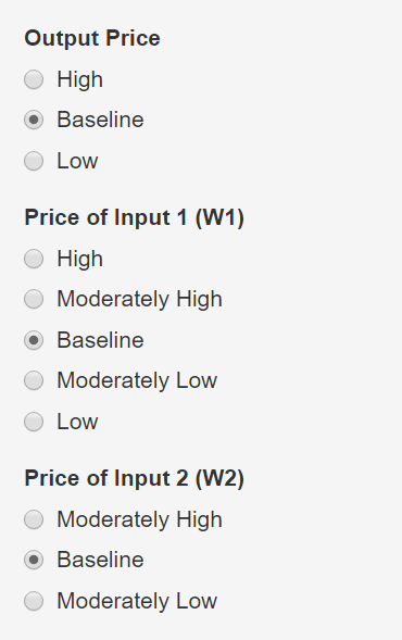
Demonstration \(\PageIndex{1}\) will be used to help you understand input demand. The top panel of the demonstration presents an isoquant map very similar to that shown in above in Figure \(\PageIndex{2}\), the bottom panel shows this firm’s demand curve for the input \(x_{1}\). As you use this demonstration, note that the profit maximizing production plan always occurs at a point where the isoquant is tangent to the isocost line. This reflects the fact that the firm is simultaneously choosing its inputs to minimize the cost of obtaining the desired output. Step through this demonstration by doing each of the following:
Focus first on the top panel of the demonstration. Increase only the output price from “baseline” to “high”. You will notice that the profit maximizing quantity shifts in a northeasterly direction to a higher isoquant when you do this. Now, decrease the output price back to the baseline and then to low. You see the isoquant shift in a southwesterly direction to lower levels of output. What you are seeing in the top panel is simply the law of supply. The firm’s profit maximizing production plan involves more output at a higher output price than at a lower output price.
Set the output price and the price and the price of input 2 to “baseline”. Set the price of input 1 to “high”. Now, gradually drop the price of input 1 through each price level until you reach “low”. As you do, pay attention to the relationship between the top panel and the input demand curve in the bottom panel. The input demand curve in the bottom panel simply reflects the profit maximizing production plans from the top panel. Thus, you see that the demand for the input is derived from the profit maximizing behavior of the firm. Note that this input demand satisfies the law of demand as presented in Chapter 1. At lower input prices more is demanded and vice versa.
Return all values to their baseline level. Now shift the output price from high to low. What happens to the demand schedule for \(x_{1}\)? You should see it shift. Similarly, increase and decrease the price of input 2. You will similarly see a shift in the demand schedule for \(x_{1}\). The takeaway here is that changes in the output price or the price of other inputs will shift the demand for an input. An increase in output price will always increase the demand for an input, all else equal. In this particular example, an increase (decrease) in the price of input 2, shifts the demand for input 1 inwards (outwards).
Finally, return all values in the demonstration to their baseline levels. Now set the price of input 1 to “low” and the price of input 2 to “moderately high”. Compare the resulting production plan to the baseline plan, denoted by point B in the top panel of the demonstration. Notice that the new production plan involves a large increase in \(x_{1}\) relative to the baseline. The point to be made here is that the optimal production plan will favor lower-priced inputs. You should have noticed that the slope of the isocost line became flatter, which shifted points of tangency to the right in favor of \(x_{1}\).
Demonstration \(\PageIndex{1}\): Deriving the inverse demand schedule for an input from a firm’s profit maximizing behavior.
Capital and Labor Intensity in Agriculture: A Case Example
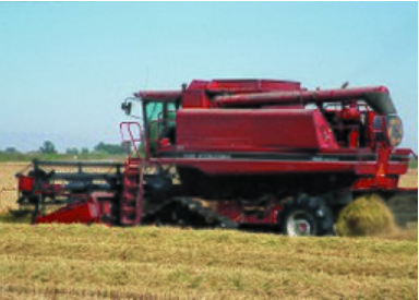
Figure \(\PageIndex{3}\) shows two methods of harvesting rice. The photo on the left is from Bhutan the photo on the right is from the United States. The method being used in Bhutan is labor intensive. The method being used in California is capital intensive. Which method is the best?
Figure \(\PageIndex{3}\): Labor and capital intensive methods of harvesting rice.
Photo on the left by Steve Evans from Citizen of the World (Bhutan) CC BY 2.0, via Wikimedia Commons. Photo on the right by Gary Kramer courtesy of USDA Natural Resources Conservation Service., via Wikimedia Commons.
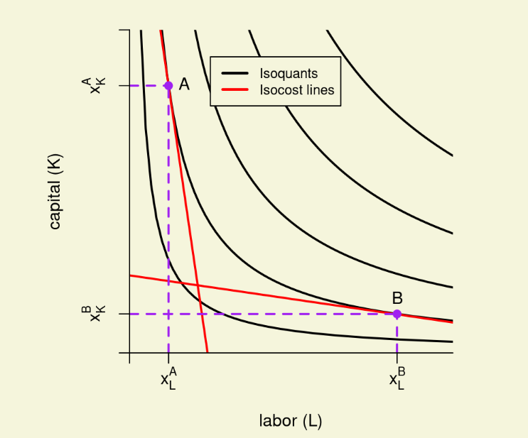
Given the concepts above, a case can be made that each method is probably best given the prices of the two inputs (labor and capital) in Bhutan and the United States. In Bhutan, labor is inexpensive relative to capital. In the United States, the reverse is true. This can be represented on the isoquant/isocost map in Figure 6. The optimal production plan in Bhutan would occur at a point like B, where the slope of the isoquant is relatively flat to match the small labor to capital price ratio. The isocost line in the United States is much steeper. Consequently, an optimal production plan for US rice harvest would occur at a point where the isoquant is equally steep, such as point A in Figure \(\PageIndex{4}\).
Figure \(\PageIndex{6}\): Labor and capital intensive production plans.