The Carte Blanche Principle says that cash is always as good as or better than in-kind. There is a corollary from the public finance literature: Lump sum taxes are better than quantity taxes.
Public finance is a field of economics that studies the role of government in the economy. Budgeting, collecting taxes, and government spending are some of the areas studied by public finance economists.
There are, of course, many different kinds of taxes. A lump sum tax is a fixed amount that must be paid, regardless of how much is purchased. A head tax, where a fee is charged to each person, is an example of a lump sum tax.
A quantity tax is an amount for each unit sold so it is added to the price of the product. Federal, state, and local governments levy quantity taxes on gasoline, alcoholic beverages, and tobacco. Unlike a lump sum tax, if more is bought, more quantity tax is paid.
Most people are familiar with sales tax, but this is yet another tax variant. Like a quantity tax, more is paid as more is purchased, but a sales tax is a percentage of the total purchase value. This is an ad valorem tax, which is Latin for "according to value."
The goals of taxation can be complicated. The primary motivation for taxes is to pay for government spending, but taxes can also be used to discourage particular activities. Both of these motivations are at play in the case of cigarettes.
Cigarette Smoking and Taxes
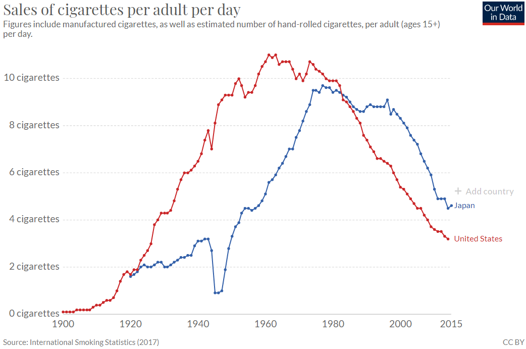
The average number of cigarettes sold per day in the United States and Japan since 1900 is shown in Figure 3.16. Visit ourworldindata.org/smoking to see an interactive version of this chart and add other countries. The pattern is the same around the worldrising smoking rates reach a peak, then a rapid decline.
Figure 3.16: Smoking rates in Japan and the United States.
American soldiers were given cigarettes during the two world wars and this drove the sharp increase in cigarette smoking. The collapse in its smoking rate in the 1940s shows that Japan did not do this. In both countries, awareness of the damaging health effects of smoking triggered the decline.
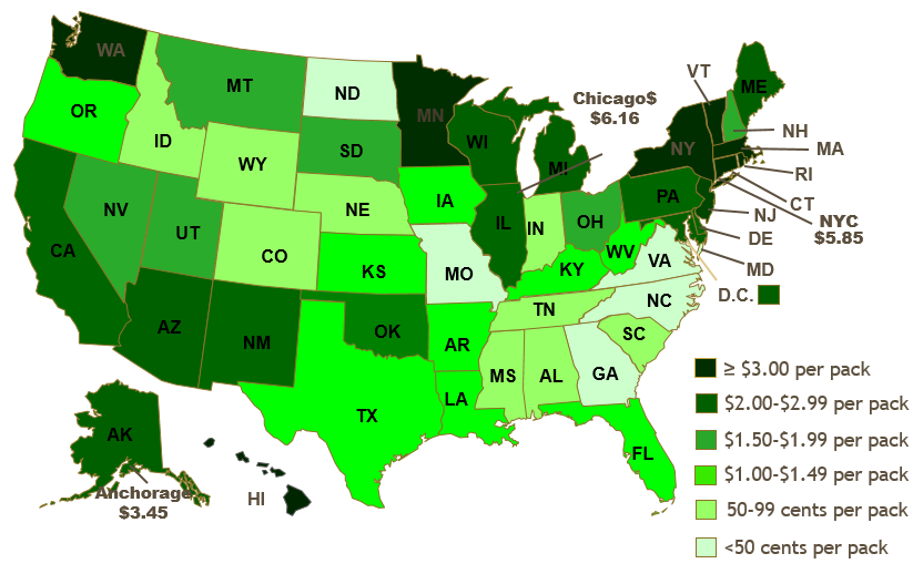
As consumption underwent this long rise and fall, cigarette tax policies also changed dramatically. Tobacco products have always been taxed, but cigarette taxes have risen dramatically in the last few decades. Figure 3.17 shows tax rates in US states in 2019.
Figure 3.17: State cigarette quantity taxes in 2019.
There is wide variation in state cigarette tax rates. In 2019, New York and Connecticut had the highest state tax of $4.35 per 20-pack of cigarettes. Missouri had the lowest, $0.17 per pack.
Other governmental levels also tax cigarettes. New York City, for example, adds a $1.50 per pack tax, bringing state and local taxes to $5.85 per pack. To this we add the federal tax rate of $1.0066 per pack. Finally, smokers pay a sales tax on the total price paid (including the quantity taxes). In New York City, a pack of cigarettes cost over $10 in 2019.
We will analyze the quantity tax by using the Theory of Consumer Behavior. We will also compare it to a lump sum taxan option that is not currently being used by the government. To make a good comparison, we have to make sure that the taxes are revenue neutral. This means that the tax revenues generated by the tax proposals are the same. It would not be fair to compare a quantity tax that generated $50 in revenues to a $100 lump sum tax.
Quantity Tax
STEP Open the Excel workbook CigaretteTaxes.xls, read the Intro sheet, and proceed to the QuantityTax sheet.
Cell B21 enables us to levy a quantity tax. The sheet opens with cell B21 = 0, which means there is no tax.
The sheet also opens with the consumer considering the bundle 20,60. The MRS is greater than the price ratio (in absolute value) and the consumer can move down the budget constraint so we know utility is not being maximized.
STEP Utility is maximized at 1250 by consuming 25 units of cigarettes (\(x_1\)) and 50 units of other goods (\(x_2\)). Run Solver to confirm this result.
Suppose we impose a $1/unit quantity tax on cigarettes. What effect does this have on the consumer?
STEP You can find the consumer’s optimal solution after levying the tax by changing cell B21 to 1 and running Solver.
Notice how the chart updated when B21 was set to one. The red budget constraint shows how the line rotated and swung in when the tax was imposed. This is the same as increasing the price of good 1. After running Solver, you can see that the consumer responds by buying fewer cigarettes.
We can also find the optimal solution using analytical methods by solving the following constrained optimization problem: \[\max\limits_{x_1,x_2,\lambda}U(x_1,x_2) = x_1x_2 \\ \textrm{s.t. } 100 = 2(x_1 + Q\_Tax) + x_2\] The consumer wishes to maximize utility (which is Cobb-Douglas with both exponents equal to 1), subject to the budget constraint, with parameter values for income and prices plugged in.
We leave \(Q\_Tax\) as an exogenous variable so we can find the optimal solution as a function of \(Q\_Tax\). We have worked on this problem before, except \(p_2 = 1\) (instead of 3) and we have added the quantity tax.
The Lagrangean procedure remains the same and we walk through the four steps to find the answer.
1. Rewrite the constraint so that it is equal to zero.
\(0 = 100 - 2(x_1 + Q\_Tax) - x_2\)
2. Form the Lagrangean function.
Notice that we are working with a mixed concrete and general problem. We have numerical values for prices, income, and the utility function exponents, but we have the amount of the quantity tax as a variable. We use this strategy whenever we want to find the optimal solution as a function of a particular exogenous variable.
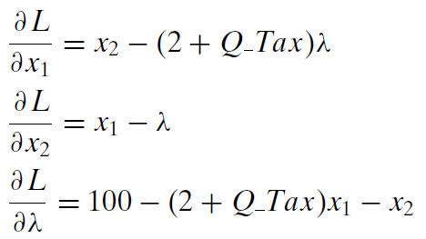
3. Take partial derivatives with respect to \(x_1\), \(x_2\), and \(\lambda\).
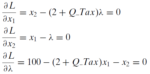
4. Set the derivatives equal to zero and solve for \(x_1\mbox{*}\), \(x_2\mbox{*}\), and \(\lambda\mbox{*}\).
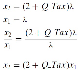
We use the usual solution method, moving the lambda terms to the right-hand side and then dividing the first equation by the second, which allows us to cancel the lambda terms.
Finding an expression for \(x_2\) seems like an answer, but it is not because it is a function of \(x_1\). To be a solution (which is called a reduced form), we must solve for \(x_1\) asa function of exogenous variables alone. We must keep working. Canceling the lambda terms has moved us closer to an answerwe have reduced the three equation, three unknown system to two equations in two unknowns.
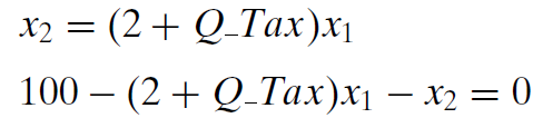
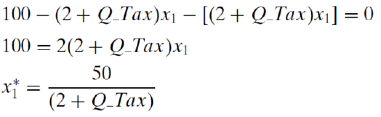
We substitute the first equation into the second and solve for the optimal amount of good 1.
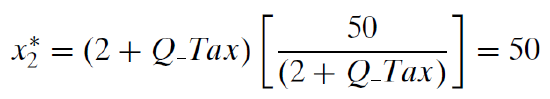
Then, we substitute this into our expression for \(x_2\) to get the optimal amount of good 2.
We can check this solution with Solver’s result by substituting \(Q\_Tax = 1\) into the reduced form solution for the two goods. Optimal cigarette consumption is \(\frac{50}{3}\) or \(16 \frac{2}{3}\). Because \(Q\_Tax\) does not appear in the optimal solution for good 2, its value is simply 50 for any value of \(Q\_Tax\).
Lump Sum Tax
Let’s see how the consumer would optimize with a lump sum tax that raised the same tax revenue for the government.
STEP Making sure that you have run Solver in the Quantity sheet with B21 = 1 so that B11 is approximately \(16 \frac{2}{3}\), proceed to the LumpSumTax sheet.
The quantity tax imposed in the QuantityTax sheet has been replaced with a revenue-neutral lump sum tax. With a $1/unit quantity tax, the consumer purchases \(16 \frac{2}{3}\) units of \(x_1\), which means the state generates $16.67 of revenue from the quantity tax. It could have generated the same revenue by taxing the consumer $16.67, regardless of how much \(x_1\) or \(x_2\) the consumer bought. This is called a lump sum tax because you pay a fixed amount (that’s the “lump sum” part) no matter what you decide to buy.
The difference in the way the lump sum tax operates is reflected in the budget constraint equation. Instead of being part of the price of good 1 like a quantity tax, the lump sum tax is subtracted from income. \[100 = 2(x_1 + Q\_Tax) + x_2\\ 100 - Lump\_Tax = 2x_1 + x_2\] The two charts show how the lump sum tax works differently than the quantity tax. Instead of rotating, the new budget line (in red) in the LumpSum sheet has shifted inwards. How would the consumer respond to this tax?
STEP Run Solver to find the optimal solution with the lump sum tax.
Before we compare the quantity and lump sum tax solutions, we confirm Solver’s answer in the LumpSum sheet by solving the problem analytically.
STEP Try your hand at this problem. Check your work (or peek if you get stuck) by clicking the button.
Remember, Solver gave you an answer so can be quite sure you are correct if your analytical work gives the same result.
Comparing Quantity and Lump Sum Taxes
We now have the data needed to compare the two tax schemes, as shown in Figure 3.18.
Figure 3.18: Comparing the tax schemes.
The first row shows that the consumer will buy the bundle 25,50 when there is no tax, generating an optimal utility of 1250. Obviously, there is no revenue because there is no tax.
The second row shows that utility falls to \(833 \frac{1}{3}\) with an optimal solution of \(16 \frac{2}{3}\),50 with a $1/unit of \(x_1\) quantity tax. The tax produces $16.67 of revenue for the government.
The last row shows that a revenue-neutral lump sum tax of $16.67 would result in purchases of \(21 \frac{5}{6}\) and \(41 \frac{2}{3}\), which would give a level of utility of 868.
The primary lesson is that, for this consumer, if the government needed to raise $16.67 of tax revenue, the lump sum tax is better than the quantity tax because the consumer’s maximum utility is higher under the lump sum tax.
Notice that we are not violating the rule against interpreting utility values as being meaningful. We are not comparing two consumers. We are not treating utility as if it were on a cardinal scale by saying, for example, that there is a gain of 868 minus \(833 \frac{1}{3}\) equals \(34 \frac{2}{3}\) utils of increased satisfaction. We are merely saying that satisfaction is higher under the lump sum tax scheme than the revenue-neutral quantity tax.
A graph can be used to explain this rather curious result that lump sum taxes enable higher utility than equivalent revenue quantity taxes. It is a complicated graph, so we will build up to it in stages.
The first layer is simply the initial solution, before any tax is applied. It is shown in Figure 3.19.
3.19: The initial optimal solution.
Figure 3.20 shows what happens with a quantity tax. The budget constraint rotates in because the price paid by the consumer (composed of the price of the product plus the tax) has increased. The consumer is forced to re-optimize and find a new optimal solution, labeled Quantity Tax. Utility has clearly fallen since we are on a lower indifference curve.
Figure 3.20: Applying a quantity tax.
Then we add a final layer to show the lump sum tax, as shown in Figure 3.21. This enables comparison of the two tax schemes.
Figure 3.21: Adding a lump sum tax.
The lump sum tax budget constraint has to go through the optimal choice bundle with the quantity tax so that the lump sum tax raises the same revenue as the quantity tax. It also has to be parallel to the original budget constraint. Because it cuts the indifference curve at the quantity tax’s optimal solution, we know we can move down the budget line and reach a higher indifference curve than the quantity tax solution.
Figure 3.21 shows that, starting from the Original Choice point, we can compare a quantity tax and a revenue-neutral lump sum tax. Figure 3.21 makes clear that the lump sum tax enables attainment of a higher level of utility than the quantity tax because the indifference curve attainable under the lump sum tax is higher than the indifference curve that maximizes utility with the quantity tax.
The reason why the lump sum tax is better is due to the fact that it is non-distorting. It leaves the relative prices of the two goods unchanged.
The Lesson and a Follow-up Question
The lesson is that the Theory of Consumer Behavior has been used to show that lump sum taxes are better than quantity taxes. Generating the same amount of revenue, lump sum taxes enable the consumer to reach a higher level of satisfaction than quantity taxes.
This begs a question: Why do we see quantity taxes instead of lump sum taxes? Why are cigarettes (and alcohol and gasoline) so heavily quantity taxed?
The answer lies in the diversity of consumers. The lesson holds only for each individual consumer. It is a fact that there is a revenue-neutral lump sum tax that leaves each individual consumer better off. The amount, however, of the preferable lump sum tax is different, in general, for each consumer. It depends on how many cigarettes (or alcohol or gasoline) each consumer buys. In other words, the lesson does not hold for all consumers taken as a whole. Thus, a single lump tax for all consumers will not necessarily yield higher utility than a quantity tax for each consumer.
This point is obvious if you consider a consumer who does not buy the taxed product at all. This consumer would prefer any size quantity tax to a lump sum tax. After all, if you do not smoke, you do not have to pay any quantity tax on tobacco. The collapse in smoking (see Figure 3.16) goes a long way to explaining why cigarette taxes have soared.
Lump Sum Corollary to the Carte Blanche Principle
We used the Theory of Consumer Behavior to demonstrate a corollary to the Carte Blanche Principle: for consumers of a particular product, a lump sum tax is better than a revenue-neutral quantity tax.
If given the option between a quantity and a revenue-neutral lump sum tax, a consumer who buys the taxed good would prefer the lump sum tax because it will leave the consumer with a higher level of utility. Unlike the quantity tax, the lump sum tax will not distort the relative prices faced by the consumer.
Although the Lump Sum Corollary is true, we see quantity taxes for various products because the Lump Sum Corollary does not apply to all consumers taken as a group. It is not true that there is a single lump sum tax that is preferred to a quantity tax by all consumers.
Exercises
Return to the CigaretteTaxes.xls workbook and apply a $2/unit quantity tax. Run Solver. Find the solution by evaluating the reduced form. Show your work. Do the two methods agree?
Repeat this for the lump sum tax. Find the revenue-neutral solution via Solver, evaluate the reduced form expression at the new Lump_Tax, and compare the two methods. Do the two methods agree?
Would the percentage change in the consumer’s consumption of \(x_1\) be more affected by a quantity tax if her indifference curves were flatter, assuming a Cobb-Douglas utility function? Describe your procedure in answering this question.
References
The epigraph is from the online version of The Wealth of Nations by Adam Smith, who is well known as the father of economics. You can access The Wealth of Nations (and many other texts) online at www.econlib.org/. If you want a physical copy of the book, used copies abound or you can get a new, inexpensive copy at www.libertyfund.org/.
Cigarette sales data were obtained from Hannah Ritchie and Max Roser (2020) "Smoking," published online at ourworldindata.org/smoking. Our World in Data is a website with striking, thought-provoking data visualizations on a range of topics.
The state tax map is from Frank J. Chaloupka’s PowerPoint presentation, "The Truth about Tobacco Economics," available at tobacconomics.org/. Tobacco data, research, and news from around the world makes this a good source for information on smoking and tobacco policy.
The Centers for Disease Control and Prevention publishes data from 1970 on state-level cigarette prices and taxes from the Tax Burden on Tobacco.
Finally, e-cigarettes are also taxed. Cotti, Chad D., Charles J. Courtemanche, Johanna Catherine Maclean, Erik T. Nesson, Michael F. Pesko, and Nathan Tefft (January 2020), "The Effects of E-Cigarette Taxes on E-Cigarette Prices and Tobacco Product Sales: Evidence from Retail Panel Data," NBER, www.nber.org/papers/w26724. From the abstract, "We then calculate an e-cigarette own-price elasticity of \(-2.6\) and a positive cross-price elasticity of demand between e-cigarettes and traditional cigarettes of 1.1, suggesting that e-cigarettes and traditional cigarettes are economic substitutes."


 button.
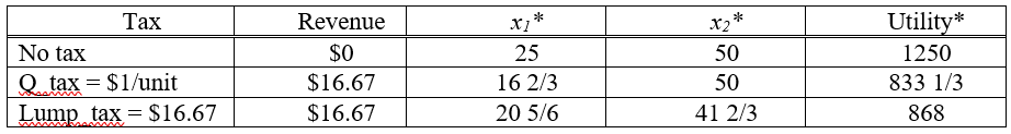 Figure 3.18: Comparing the tax schemes.
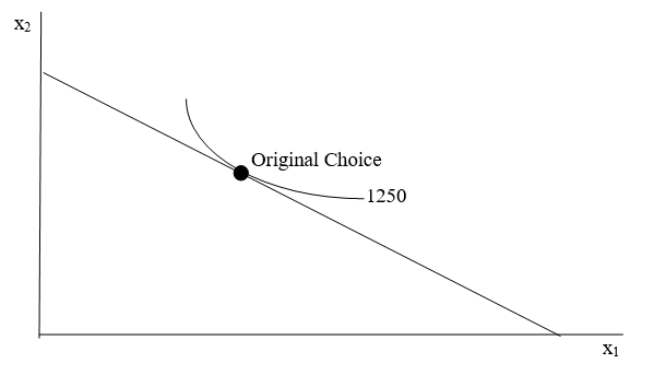 3.19: The initial optimal solution.
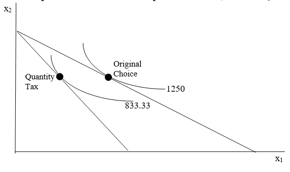 Figure 3.20: Applying a quantity tax.
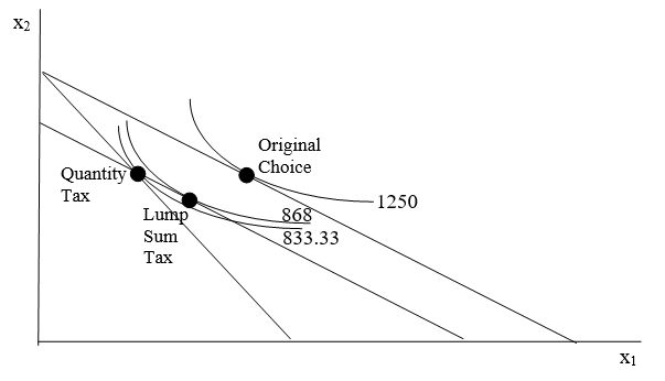 Figure 3.21: Adding a lump sum tax.