Like the perfectly competitive firm, a monopolist has three interrelated optimization problems. Attention is focused on the output profit max problem because that is where the essential difference lies between a perfectly competitive (PC) firm and a monopoly. We know that via consistency, monopoly power manifests itself on the input side also. A monopoly will produce less than a PC firm and, in turn, hire less labor and capital.
Unlike a PC firm, a monopoly chooses output and the price at which to sell the product. This makes the monopoly problem harder to solve. Fortunately, your experience with optimization, comparative statics, and graphical displays give you the background needed to understand and master monopoly.
Definition and Issues
A monopoly is defined as a firm that is the sole seller of a product with no close substitutes. The definition is inherently vague because there is no clear demarcation for what constitutes a close substitute.
Consider this example: In the old days, a local cable provider might have an exclusive agreement to provide cable TV in a community. One could argue that the cable provider was a monopoly because it was the sole seller of cable TV. But what are the substitutes for cable TV?
Years ago, cable TV was the only way to access subscription channels such as ESPN and HBO. Commercial broadcasts (with national broadcasters such as ABC, NBC, and CBS and local channels) were a poor substitute for cable TV. In this environment, cable TV would be a good example of a monopoly.
Today, however, cable TV has strong competition from satellite services and streaming services from the web. Even if a firm had an exclusive franchise to deliver cable TV in a community, there are many ways to get essentially the same package of channels. Today, cable TV is not a monopoly.
Of course, cable TV is not a good example of perfect competition either. The cable company does not accept price as a given variable. It is in the middle, somewhere between perfect competition and monopoly. Markets served by a few firms are called oligopolies. Add more firms and you eventually get monopolistic competition. The study of how firms behave under a variety of market structures is part of the subdiscipline of economics called Industrial Organization. Figure 15.1 sums things up.
Figure 15.1: A continuum of market structures.
Barrier to Entry
To remain a monopoly, the firm must have a barrier to entry to prevent other firms from selling its product. In the cable TV example, the barrier to entry was provided by the exclusive agreement with the community. Such governmental restriction is a common form of a barrier to entry.
Another way to erect a barrier to entry is control over a needed input. ALCOA (the Aluminum Corporation of America) had a monopoly in aluminum in the early 20th century because it owned virtually all bauxite reserves.
If a product requires entry on a large scale, like automobile manufacturing, this is considered a barrier to entry. To compete against established car companies, a firm must not only produce cars, but also many spare parts and figure out how to sell the product.
Like the concept of a close substitute, a barrier to entry is not a simple yes or no issue. Barriers can be weak or strong and they can change over time. Cable TV’s barrier was eroded not by changes in legal rules, but by technological changethe advent of satellite TV and the web.
Monopoly’s Revenue Function
We know that the firm’s market structure impacts its revenue function. The simplest case is a perfectly (or purely) competitive firm. It takes price as given and, therefore, revenues are simply price times quantity. For a perfect competitor, even though market demand is downward sloping, the firm’s own individual demand curve is perfectly elastic at the given, market price.
Because the PC firm can sell as much as it wants at the given price, selling one more unit of output makes total revenue (TR) increase by the price of the product. Marginal revenue (MR) is defined as the change in TR when one more unit is sold. Thus, for a PC firm, \(MR = P\).
This is not true for a monopoly. A critical implication of monopoly power is that MR diverges from the demand curve. But this is too abstract. We can use Excel to make these concepts clearer.
STEP Open the Excel workbook Monopoly.xls and read the Intro sheet, then go to the Revenue sheet to see how monopoly power affects the firm’s revenue function.
The sheet opens with a perfectly competitive revenue structure. Total revenue is a linear function of output and, therefore, \(P = MR\) with a horizontal line in the bottom graph. A graph with a linear TR and corresponding horizontal MR means it is a PC firm.
Unlike a PC firm, a monopoly faces the market’s downward sloping demand curve. We can model a linear inverse demand curve simply as \(P = p_0 - p_1q\). Because the slope parameter, \(p_1\), in cell T2 is initially zero, TR is linear and MR is horizontal.
STEP To show how monopoly power affects the firm’s revenue function, click on the Price Slope scroll bar.
Notice that as you increase the slope parameter, MR diverges more from D.
The smaller (in absolute value) the price elasticity of demand, the greater the divergence of MR from D and the stronger the monopoly power.
We will see that the monopolist uses the divergence of MR from D to extract higher profits than would be possible if there were other sellers of the product.
When drawing MR and D in the case of a linear inverse demand curve, keep in mind these two basic rules:
MR and D have the same intercept.
MR bisects the y axis and D.
We can derive these properties easily. With our inverse D curve, \(P = p_0 - p_1q\), we can do the following: \[TR=Pq\] \[TR = (p_0 - p_1)q\] \[TR = p_0q - p_1q\] \[MR = \frac{dTR}{dq} = p_0 - 2p_1\] Clearly, both D and MR share the same intercept, \(p_0\). Because the slope of MR is \(-2p_1\), it is twice the slope of D, which is simply \(-p_1\).
Thus, when you draw a linear inverse demand curve and then prepare to draw the corresponding MR curve, remember the two rules: (1) the intercept is the same and (2) MR has twice the slope so at every y axis value, MR is halfway between the y axis and the D curve.
Figure 15.2, with an inverse demand curve slope of \(-1\), shows the monopoly’s revenue function. Unlike the PC firm, TR is a curve and MR diverges from D. MR bisects the y axis and D. The dashed line at $20/unit, for example, shows the distance from the y axis to MR is 10, the same as MR to D.
Figure 15.2: TR, D, and MR functions for a monopolist.
Source: Monopoly.xls!Revenues
Notice that where MR = 0 at q = 20, TR is at its maximum. At this quantity, the price elasticity of demand is exactly \(-1\).
Figure 15.2 shows that MR can be negative. This can happen because there are two opposing forces at work. Increasing quantity increases TR, since \(TR= Pq\). However, the only way to sell that extra product is to lower the price (by traveling down the demand curve) so TR falls. When the increase to TR by selling additional output outweighs the effect of the drop in the price, MR is positive. Eventually, however, with a linear demand curve, the monopolist will reach a point at which the increase in revenue for selling one more unit is negative. In the range of output (\(q > 20\) in Figure 15.2) where \(MR < 0\), the effect of the decreased price outweighs the positive effect of selling more output.
When \(MR > 0\), the price elasticity of demand is greater than 1 (in absolute value). When MR is negative, demand is inelastic. The monopolist will never produce on the negative part of MR, which is the same as the inelastic portion of the demand curve.
There is a neat formula that expresses the relationship between MR and P. With an inverse demand curve, \(P(Q)\), we know that \(TR = P(Q)Q\). From the TR function we can take the derivative with respect to output to find the MR function. We use the Product Rule: \[MR=\frac{dTR}{dQ}=P+\frac{dP}{dQ}Q\] If we factor out P from this expression, then MR can be rewritten as: \[MR=P+\frac{dP}{dQ}Q=P(1+\frac{dP}{dQ}\frac{Q}{P})=P(1+\frac{1}{\epsilon})\] The Greek letter epsilon (\(\epsilon\)) is the price elasticity of demand (\(\frac{dQ}{dP}\frac{P}{Q}\)). The expression shows that \(MR = P\) under perfect competition because an individual firm faces a perfectly elastic demand curve. This means epsilon is infinite and its reciprocal is zero.
It also shows that the more inelastic the demand curve (the closer \(\epsilon\) is to 0), the greater the separation between MR and the demand curve (P). If \(\epsilon = 0\), then MR is undefined. With \(\epsilon = 0\), inverse demand is a vertical line. The monopoly would charge an infinite price.
Setting Up the Problem
There are three parts to every optimization problem. Here is the framework for a monopolist’s output side profit maximization problem.
Goal: maximize profits (\(\pi\)), which equal total revenues (TR) minus total costs (TC).
Endogenous variables: output (q) and price (P)
Exogenous variables: input prices (the wage rate and the rental rate of capital), demand function coefficients, and technology (parameters in the production function).
A monopoly differs from a PC firm only on the revenue sideprice is now endogenous. The cost structure is the same. The monopoly has an input cost min problem and it is used to derive a cost function. Increases in input prices shift cost curves up and improvements in technology shift cost curves down. The monopolist has a long and short run, just like a PC firm, and in the short run there is a gap between ATC and AVC that represents fixed costs.
Finding the Initial Solution
We will show the conventional approach to solving the monopoly problem first, then turn to an alternative formulation based on constrained optimization.
The conventional approach is to find optimal q where \(MR=MC\), then get optimal P from the demand curve, and then compute optimal \(\pi\) as a rectangle. This is the standard approach and there is a canonical graph that goes along with this approach. Its primary virtue is that it can be easily compared to the perfectly competitive case.
The conventional approach can be demonstrated with a concrete problem. Suppose the cost function is \(TC = aq^3 + bq^2 + cq + d\). Suppose the market (inverse) demand curve is \(P = p_0 - p_1q\). Thus, \(TR=Pq=(p_0-p_1)q\).
With this information, we can form the firm’s profit function and optimization problem, like this: \[\begin{gathered} %star suppresses line # \max\limits_{q} \pi = TR-TC \\ \max\limits_{q} \pi = (p_0-p_1)q - (aq^3 + bq^2 + cq + d)\end{gathered}\]
We first solve this problem with numerical methods, then analytically.
STEP Proceed to the OptimalChoice sheet and look it over.
The profit function has been entered into cell B4. Quantity and price are displayed as endogenous variables, but q is bolded to indicate that it is the primary endogenous variable. In other words, Solver will search for the profit-maximizing output and, having found it, will compute the highest price that can be obtained from the demand curve.
The firm is making $245 in profits by producing 10 units of output and charging $34.50 per unit, but this is not the profit-maximizing solution. We know this because the marginal revenue of the 10th unit is $29/unit, whereas the marginal cost of that last unit is only $4/unit. Clearly, the firm should produce more because it is making more in additional revenues from the last unit produced than the additional cost of producing that unit.
STEP Run Solver to find the optimal solution.
At the optimal solution, the equimarginal condition, \(MR = MC\), is met. With positive profits, this is a clear signal that we have found the answer.
Before you click the button, try doing the problem on your own. This is a single variable unconstrained maximization because \(P = p_0 - p_1q\) has been substituted into the profit function. Take the derivative with respect to q, set it equal to zero, and solve for optimal q. Substituting in the parameter values to make it a concrete problem makes it easier to do the math: \[\begin{gathered} %star suppresses line # \max\limits_{q} \pi = (40-0.55)q - (0.04q^3 - 0.9q^2 + 10q + 50)\end{gathered}\]
You can check your work by clicking the button. You can also confirm that the two approaches, Solver and calculus, agree.
STEP Proceed to the OutputSide sheet to see a familiar set of four graphs.
As usual, the totals are on the top and the average and marginal curves on the bottom. The cost curves are the quite similar to the PC firm’s output profit maximization graphs, but the revenue curves are quite different.
The bottom left-hand corner graph in Figure 15.3 is the canonical graph for a monopolist. It can be used to quickly find \(q \mbox{*}\), \(P \mbox{*}\), and \(\pi \mbox{*}\). Here’s how to read and use the conventional monopoly graph:
Finding \(q \mbox{*}\): Choose q where \(MR = MC\). This gives the biggest the difference between TR and TC and puts you on top of the profit hill (in the top right graph).
At \(q \mbox{*}\), travel straight up until you hit the demand curve to get \(P \mbox{*}\). This is the highest price that the monopolist can get for the chosen level of output.
Create the usual profit rectangle as \((AR – ATC)q \mbox{*}\). It has length \(q \mbox{*}\) and height \(AR - ATC\) (where \(AR = P\)). The area of this rectangle equals the distance of the line segment between TR and TC, which is the height of the profit hill.
Play with the slider controls to improve your understanding of the graphs and relationships.
STEP Click the Fixed Cost slider to manipulate total fixed costs (d in the cubic cost function).
Changes in fixed costs do not affect the monopolist’s optimal quantity and price solution. This is just like the perfectly competitive case.
STEP Click the button; explore changes in the price intercept to see how the firm responds. At a low enough price intercept, profits become negative and, just like a PC firm, if \(P < AVC\), the firm will shut down.
You can also control the firm’s monopoly power by manipulating the inverse demand curve’s slope.
STEP Set the Price Slope slider to zero. What happens?
You stripped the monopoly of its price power and it is a PC firm.
No Supply Curve for Monopoly
Monopolists do not have a supply curve. This seems like a strange statement since monopolies produce output and so "supply" whatever good or service of which they are the sole seller. But the key lies in the definition of a supply curve: given price, the supply curve gives the quantity that will be produced.
Because a PC firm is a price taker, it is possible to shock P and see how the optimal output changes. We can derive \(q \mbox{*} = f(P, \textrm{ ceteris paribus})\) and this is called a supply curve.
Unlike a perfectly competitive firm, for which price is exogenous, a monopoly chooses the price. Thus, we cannot ask, "Given this price, what is the optimal quantity supplied?" With price as an endogenous variable, it cannot serve as a shock variable in a comparative statics analysis.
We can (and you just did) shock a monopolist’s demand curve parameters such as the intercept and slope, but this is not an exogenous change in the price of the product. The experiment of changing the price cannot be applied to a monopolist and, therefore, the monopolist has no supply curve.
Measuring Monopoly Power
Another common misconception is that monopoly is either zero or one. In fact, it is a continuum and you can have more or less monopoly power. There are several ways to measure it.
STEP Proceed to the Lerner sheet.
This sheet demonstrates the point that the more inelastic the demand faced by a monopolist, the greater the monopoly power. In other words, from a profit-maximizing point of view, it is better to have a monopoly over a product that everyone desperately needs (i.e., very inelastic) than to be the sole seller of a product that has a highly elastic market demand curve.
Abba Lerner formalized this idea in a mathematical expression that bears his name, the Lerner Index. "If P = price and MC = marginal cost, then the index of the degree of monopoly power is \(\frac{P-MC}{P}\)." (Lerner, 1934, p. 169). This measure of monopoly power uses the gap between P and MC as a percentage of P.
The Lerner Index takes advantage of the fact that a monopolist will choose that quantity where \(MR = MC\), then charge the highest price possible for that quantity. The higher the price that can be charged, the more inelastic is demand and the greater the monopoly power.
The Lerner sheet compares two monopolies with the exact same cost structure (assumed for simplicity to have a constant \(MC = AC\)). They both produce the same profit-maximizing quantity, but Firm 2 faces a more inelastic demand curve than Firm 1 and, therefore, it has a bigger gap between price and marginal cost.
STEP Click on cells B16 and I16 to see the simple formulas for the Lerner Index.
The idea is that the bigger the divergence between price and marginal cost, the greater the monopoly power. Firm 2 has more monopoly power than Firm 1 and more monopoly profits. The Lerner Index for each firm reflects this.
Notice that a perfectly competitive firm that sets \(MC = P\) will have a Lerner Index of zero. As the index approaches one, monopoly power rises.
STEP Change Firm 2’s demand parameters to 130 for the intercept and 20 for the slope. The y axis is locked down so the entire D and MR functions are not displayed.
The optimal quantity is still 3, but P and profits are higher, as is the Lerner Index.
STEP Make the demand curve more inelastic at \(Q=3\) by setting the demand parameters to 190 and 30.
Optimal P has increased again, along with profits. The Lerner Index reflects the greater monopoly power.
STEP One last time, change the demand parameters to 6010 and 1000. The graph is hard to read because only MR is shown; D is literally off the chart.
Firm 2 continues to produce the same output as Firm 1, but has a much, much higher optimal price and maximum profits. Its Lerner Index is close to one. It cannot rise above one, but the closer it gets, the greater the divergence of P and MC so the greater the monopoly power.
The Lerner sheet also shows that the Lerner Index can be expressed as the reciprocal of the price elasticity of demand at the profit-maximizing price. The few algebra steps needed to connect the Lerner Index to the price elasticity start in row 25.
STEP Set Firm 2’s demand parameters back to 70 and 10, and then click the button.
The price elasticity of demand for the two firms is displayed. If you click in the cells, you can see the formula. Notice that the reciprocal of the inverse demand curve’s slope is used to compute the price elasticity of demand correctly.
Firm 2’s price elasticity of demand at the profit-maximizing price is lower than Firm 1’s. The lower the price elasticity and the higher the Lerner Index, the greater the firm’s monopoly power.
STEP Proceed to the Herfindahl sheet for a quick look at another way to measure monopoly power.
Instead of measuring the markup of price over marginal cost, we can see how big the firms are in an industry. Strictly speaking, a monopoly is one firm so it would have a 100% market share, but in practice, firms have monopoly power even though they are not technically monopolies. Any firm that faces a downward sloping demand curve and has the ability to set its price is said to have monopoly power.
If a market has many firms, each with the same share of total sales, we have a competitive market structure. If, on the other hand, only a few firms exist, the market is monopolized. The question is how to measure the degree of monopolization?
We can sort the firms in an industry from highest to lowest share and then add the shares of the four biggest firms. This gives the four firm concentration ratio in cell D5. It turns out this is not a very good way to distinguish between concentrated and unconcentrated industries.
The problem is that the four firm concentration ratio tells you nothing about the sizes of the top four firms or the rest of the market. The four firm concentration ratio is 70%, which seems pretty highly concentrated. The biggest firm’s share, 30%, is almost one-third of the entire industry.
STEP Click on the button.
The four firm concentration ratio is the same as before (70%), but this industry is clearly much more concentrated. Firm A is even bigger and the others are tiny.
STEP Click on the button.
The four firm concentration ratio is the same as before (70%), but this industry is clearly less concentrated. The four top firms are equal so no one firm really dominates.
The primary virtue of the four firm concentration ratio is that it is easy to compute and understand. However, because we have three scenarios with wildly different shares for the top four firms yielding the same four firm concentration ratio, we can conclude that this ratio is a poor way to determine whether firms in a market are in a competitive or monopolistic environment. The four firm concentration ratio might be easy to compute and understand, but it is incapable of picking up differences in the distribution of shares.
A better way to judge concentration is via the Herfindahl Index. Unlike the Lerner Index, there is confusion about who invented it. Hirschman concludes, “The net result is that my index is named either after Gini who did not invent it at all or after Herfindahl who reinvented it. Well, it’s a cruel world” (Hirschman, 1964, p. 761). It is sometimes called the Herfindahl-Hirschman Index (HHI).
Fortunately, its computation is simpler than its paternity. The idea is to square each share and sum, like this: \[H=\sum_{i=1}^{n}S_i^2\] The index ranges from 1/n to 1 (when using decimal values of shares). The higher the index, the greater the concentration. By squaring the shares, it gives more weight to bigger firms: for example, \(0.1^2 = 0.01\), while \(0.3^2=0.09\).
The Herfindahl sheet shows the computation. Notice how each value in column B is squared in column G. The sum of the squares is in cell G15 and it is the value of the Herfindahl Index.
STEP Click on the three buttons one after the other to cycle through them. Notice how the Herfindahl Index changes (but the four firm concentration ratio does not).
For Distribution A, the H value is 0.325. This is quite high. The 0.1375 value with Distribution B means there is more competition in this scenario than the other two.
The Herfindahl Index is not perfect because no single number can completely describe an entire distribution. It is, however, better than the four firm concentration ratio and often used to measure the degree of market competition.
The United States Department of Justice is charged with regulating the conduct and organization of businesses. The mission of the Antitrust Division is to promote economic competition. They use the Herfindahl Index as part of their Horizontal Merger Guidelines (www.justice.gov/atr/horizontal-merger-guidelines-08192010). Markets with a Herfindahl Index less than 0.15 are "unconcentrated," values between 0.15 and 0.25 are "moderately concentrated," and anything over 0.25 is "highly concentrated."
The Department of Justice deems any proposed merger that increases the Herfindahl Index by more than 0.01 (100 points in the scale they use) in concentrated markets as warranting scrutiny. They can go to court to block mergers to prevent too much concentration. They can also break up companies that have too much monopoly power. This is known as antitrust law and is part of the Industrial Organization field of economics.
An Unconventional Approach
The monopolist’s profit maximization problem can also be solved by choosing P and q simultaneously subject to the constraint of the demand curve. While this is not the usual way of framing the monopoly’s optimization problem, it enables practice with the Lagrangean method of solving constrained optimization problems and reading isoprofit curves.
The analytical solution is based on rewriting the constraint so it is equal to zero (\(P-(p_0-p_1q)=0\)), forming the Lagrangean, setting derivatives equal to zero, and solving the system of equations for the optimal solution.
Set each derivative equal to zero and solve the three first-order conditions for \(q \mbox{*}\), \(P \mbox{*}\), and \(\lambda \mbox{*}\). From the first equation, \(\lambda = -q\), substitute into the second equation: \[P - 3aq^2 - 2bq - c + [-q] p_1 = 0\] From the third first-order condition, \(P = p_0 - p_1q\), so \[(p_0 - p_1q) - 3aq^2 - 2bq - c - qp_1 = 0\] Rearrange the terms to prepare for using the quadratic formula.
STEP Proceed to the ConOpt sheet to see formulas based on the Lagrangean solution starting in cell F24.
Naturally, we get the same, correct answer as the unconstrained version.
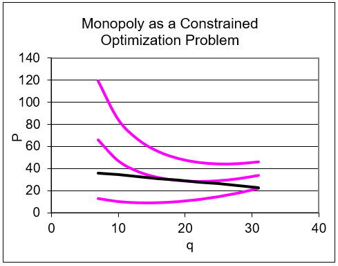
The ConOpt sheet shows that monopoly as a constrained optimization problem can be depicted with a graph. The pink curves are isoprofit curves and the black line is inverse demand. The MR curve is not drawn because it is not used. The firm is trying to get to highest isoprofit without violating the demand curve constraint. Clearly, the opening values are not optimal.
STEP Run Solver and get a Sensitivity Report to confirm the value of lambda star is minus optimal quantity. Notice how the Solver dialog box is set up so Solver chooses cells B8 and B9 subject to the constraint.
After running Solver, the graph, reproduced in Figure 15.4, shows the usual tangency result.
Figure 15.4: The constrained optimization version of the monopoly problem.
Source: Monopoly.xls!ConOpt
The point of tangency provides the optimal q and P solution, while the value of the isoprofit curve at that point is the level of profits.
Do not be confused. The constrained version is rarely used. The conventional approach is the canonical output profit maximization graph (bottom left in Figure 15,2). This graph shows the optimal q where \(MR=MC\) and easily displays \(P \mbox{*}\) from the demand curve and \(\pi \mbox{*}\) as a rectangle.
Figure 15.4 gives the same optimal solution, but presents the problem in a different way. Understanding that the demand curve serves as a constraint on monopoly is helpful. Monopoly power is not infinite. A monopolist cannot choose a ridiculously high price and a high quantity. As price rises, quantity sold must fall.
Monopoly Basics
A monopoly differs from a perfectly competitive firm in that a monopolist can choose the quantity and price, whereas a perfect competitor is a price taker. In addition, a monopolist has a barrier to entry that enables it to maintain positive economic profits even in the long run.
The two are the same, however, in the cost structure (like a perfect competitor, the monopolist derives its cost function from the input cost minimization problem) and the fact that it seeks to maximize profits (where \(MR = MC\) as long as \(P>AVC\)).
We depict the monopolist’s optimal solution with a graph that superimposes D and MR over the family of cost curves (MC, ATC, and AVC). Like a PC firm, a monopolist can suffer negative profits in the short run and it will shut down when \(P < AVC\).
Monopoly’s canonical graph (the bottom left chart in Figure 15.2) belongs in the pantheon of fundamental graphs in economics. Like the indifference curves with a budget constraint or supply and demand, a linear inverse demand with its associated marginal revenue showing optimal q (at the intersection of MR and MC, of course) and optimal P is a truly classic graph.
One way to measure monopoly power is by the Lerner Index. The greater the gap between price and marginal cost, the greater the monopoly power. The greater the price elasticity of demand, the lower the Lerner Index and the weaker the monopoly power.
The Herfindahl Index is another way to measure the strength of monopolization in a market. It measures industry concentration. Unlike the four firm concentration ratio, it uses market shares of every firm to create a single number that reflects the concentration of an industry. Mergers that boost the Herfindahl Index by more than 0.01 (100 points) in concentrated markets are carefully scrutinized by the Department of Justice because it is presumed that the market will not be competitive.
We concluded this chapter with an unconventional analysis. The monopoly’s profit maximization problem can be cast as a constrained optimization problem. In addition to providing practice with the Lagrangean method, this way of looking at monopoly makes quite clear that the monopolist must obey the demand curve.
Exercises
De Beers is an internationally famous company that had a monopoly over diamonds. Google “synthetic diamonds” to learn more. Include web citations with supporting evidence in your answers to these two questions.
What was their barrier to entry when they had a monopoly?
What happened to their monopoly?
Use Word’s Drawing Tools to depict a monopoly shutting down in the short run. Explain the graph.
In the ConOpt sheet, set the demand intercept (cell B13) to 9 and the fixed cost (B18) to 180. Run Solver. Why is Solver generating a miserable result? What is the correct answer?
Use Word’s Drawing Tools to depict the effect of monopoly from the input side profit maximization perspective. Explain the graph.
Hint: With perfect competition, \(L \mbox{*}\) is found where \(w = MRP\) (where MRP is based on the given, constant price, \(PxMP\)). With monopoly, however, P and MR diverge.
Is the effect of monopoly on the input side consistent with the effect of monopoly on the output side? Explain.
References
The epigraph is from page 149 of Hans Brems, Pioneering Economic Theory, 1630–1980: A Mathematical Restatement (1986). This book recasts ideas in the history of economics in mathematical terms. Seeing the thoughts of Smith, Ricardo, Marx, and others presented as mathematical models provides an uncommon perspective.
On the Lerner Index, see Abba P. Lerner, "The Concept of Monopoly and the Measurement of Monopoly Power," The Review of Economic Studies, Vol. 1, No. 3 (June, 1934), pp. 157–175, www.jstor.org/stable/2967480.
On the Herfindahl Index, see Albert O. Hirschman, "The Paternity of an Index," The American Economic Review, Vol. 54, No. 5 (September, 1964), p. 761, www.jstor.org/stable/1818582.


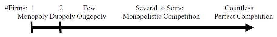 Figure 15.1: A continuum of market structures.
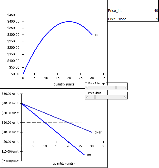
 button, try doing the problem on your own. This is a single variable unconstrained maximization because \(P = p_0 - p_1q\) has been substituted into the profit function. Take the derivative with respect to q, set it equal to zero, and solve for optimal q. Substituting in the parameter values to make it a concrete problem makes it easier to do the math: \[\begin{gathered} %star suppresses line # \max\limits_{q} \pi = (40-0.55)q - (0.04q^3 - 0.9q^2 + 10q + 50)\end{gathered}\]
 button. You can also confirm that the two approaches, Solver and calculus, agree.
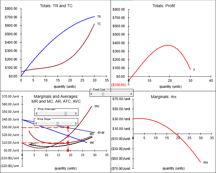
 button; explore changes in the price intercept to see how the firm responds. At a low enough price intercept, profits become negative and, just like a PC firm, if \(P < AVC\), the firm will shut down.
 button.
 button.
 button.