This section is devoted to explaining the concept of externality, why it causes a market failure, and how the inefficiency in the allocation of resources can be corrected.
The core idea is that externalities cause markets to failtoo much or too little is produced. Society’s resources are inefficiently allocated. The reason why markets fail in the presence of externalities is that decision makers (consumers or firms) fail to incorporate the full costs or benefits of an action so they make a poor decision (from society’s point of view).
There are three questions to answer:
What is an externality?
Why do externalities break the market?
How can we fix the market?
1. What is an Externality?
An externality is a cost or benefit not taken into account by the decision maker. An agent takes an action that impacts others, but she does not incorporate this “external impact” (hence the name externality) into her optimization problem. The decision maker considers only personal or private cost and benefit, not the full or social cost and benefit.
Externalities can arise on the cost or benefit side of an optimization problem. The private costs or benefits are the ones included in the agent’s calculations. The external costs or benefits are ignored. The full or total costs or benefits are called social costs or benefits.
We can better understand externalities by looking at examples. The key is always that the optimizing agent is not considering all of the costs and benefits. Costs are imposed, but not felt by the agent or benefits are conferred on others, but not captured by the agent. This leads to a privately optimal solution that diverges from the socially optimal solution and produces a misallocation of resources.
A classic example of an externality is industrial pollution. When the cost of pollution is not taken into account by the firm, this is called a negative production externality. A steel firm deciding how much steel to produce factors into its choice of output level the revenue from making steel and a whole series of costs: labor, raw materials, and equipment. The costs that are counted are private costs.
If the firm pollutes the air through a smokestack, but does not have to pay for polluting the air, this is an external cost. Social costs include private costs and external costs. It is a negative externality because costs are imposed on others that are not taken into account by the decision maker. It is a production externality because the decision is made by a firm deciding how much to produce.
A college education is another classic example of a situation where the decision maker fails to consider the total picture. It is often used to explain a positive consumption externality because there are benefits to education that are not taken into account by the student.
The choice variable is how many years of schooling to acquire beyond high school. The costs are hugeout-of-pocket costs of a 4-year college degree include tuition and books, but opportunity costs are even greater. The benefits are also quite large, including access to better jobs, higher pay, and greater quality of life. These private benefits are considered when high school students decide whether or not to go to college so they are not part of the externality.
But society benefits from education also. College-educated people have lower unemployment rates, smoke less, and are more likely to vote. These social benefits are ignored by individuals making a decision about whether or not to acquire a college education. It is a positive externality because benefits flow to others that are not taken into account by the decision maker. It is a consumption externality because the decision is made by a consumer deciding how much to purchase.
Many studies attempt to estimate the gap between the social rate of return and private rate of return to a college degree. Social rates of return to education are several percentage points higher than the private return. This gap is an estimate of the external value generated by education.
Externalities are everywhere. Some are easy to spot, like the loud music your next door neighbor plays (a negative consumption externality). To the extent that you ignore the impact on others, your decision about which shirt to wear contains an externality.
But externalities can be subtle also. Consider an army with soldiers that were drafted into service. The externality is that the government does not take into account the full cost of acquiring its soldiers. This externality disappears with a volunteer army because the military has to pay enough to entice people to join.
Externalities are all about impacts on others so it is easy to see why they are also known as spillover effects. Remember, the private costs and benefits are counted by the decision maker, but the external effects are not.
2. Why Do Externalities Break the Market?
Recall Figure 17.6, reproduced below as Figure 17.25 for your convenience.
Figure 17.25: An overall view of supply and demand.
This figure has three canonical graphs: the Theory of Consumer Behavior on the left, the Theory of the Firm on the right, and supply and demand in the middle. It says that the equilibrium solution is found at the intersection of supply and demand, which come from the firm and consumer graphs.
We can show that the equilibrium quantity equals the quantity that would maximize consumers’ and producers’ surplus. Price controls (such as ceilings or floors), taxes, and monopoly all generate market failures, defined as quantities that do not maximize CS and PS.
We can add externalities to this list. Negative externalities are costs not taken into account and they produce too much output, while positive externalities do the reverse.
Look carefully at Figure 17.25. For the market system to yield a socially desirable outcome, supply and demand must reflect the full costs and benefits of the product. But this is precisely what is not happening if an externality is present. There are positive or negative spillover effects that result in a market equilibrium that is sub-optimal.
Suppose we have a situation where producers do not take into account the costs of pollution created as a by-product of manufacturing. Then the MC curve in Figure 17.25 is not incorporating the full costs of production and the supply (which is the sum of individual MC curves) is also too low.
There is a marginal social cost, MSC, curve that does include all costs and it does yield the socially optimal solution. Figure 17.26 shows the canonical graph of a negative externality in production. It is easy to see that the marginal private cost, MPC, which firms use to decide how much to produce to maximize profits, is too low. This produces an equilibrium output that is too high.
Figure 17.26: A broken market with a negative production externality.
\(Q \mbox{*}\) in Figure 17.26 shows the optimal output for society. The socially optimal level of output is based on the full, social cost of production. \(Q_e\) shows the (broken) market’s output. The market’s equilibrium output is based only on the private cost of production so it is too high.
To sum up, a negative production externality means that firms fail to include all costs and, therefore, \(MPC < MSC\), and, therefore, \(Q_e<Q \mbox{*}\). This is why externalities cause market failure.
We can use Excel to create a simple spreadsheet that demonstrates the concepts of externality and market failure.
STEP Open the Externality.xls workbook, read the Intro sheet, then proceed to the Externalities sheet.
Let’s take a quick tour of the screen. On the left are the total and marginal graphs for a single firm. We ignore the average cost curves (ATC and AVC) because we are not interested in this firm’s profit position. All we care about is how much it will produce. The cost function is a simple quadratic and the market price is $40/unit so the revenue function is \(40q\).
On the right is the conventional supply and demand graph. Notice that the y axes of the individual and market graphs are the same. The x axes, however, are different. There are 1,000 firms and, combined, they produce tens of thousands of units of output.
Initially, this firm is producing 10 units of output. What would you advise this firm to do? Why?
STEP Use the firm’s scroll bar control to adjust its output level.
To maximize profits, this firm will choose output where \(MR = MC\). This output level will generate the maximum difference between the total revenue and total cost curves in the top graph.
The problem is easily solved via analytical methods. \[\max\limits_{q} \pi =40q-(200+q^2)\] \[\frac{d \pi}{dq} =40-2q=0 \rightarrow q \mbox{*}=20\] Both analytically and with Excel, we can see that the firm will produce 20 units when equilibrium price in the market is $40/unit. When all 1,000 firms do this we get a market equilibrium output of 20,000 units. This is the socially optimal allocation of resources to this product.
STEP To implement the externality, slide the Set Externality control all the way to the right (so the red lines and curve are above the black ones in the three graphs).
The red objects are not labeled. What do they represent?
STEP Insert text boxes to label the red curve in the top graph, the red line in the bottom graph, and the red line above the supply curve.
The correct labels must include the word social. The red line in the top graph is the total social cost, TSC, and its marginal counterpart is the marginal social cost, MSC. The divergence between the red social cost and the black private cost signals the presence of an externality. The distance between the curves are costs not taken into account by the firm.
In the market graph, the red line is MSC, by which we mean the sum of the indivdual marginal social costs. Like in the individual graph, divergence between supply and MSC is a clear marker of the presence of an externality.
Note that neither the firm’s profit-maximizing output level nor the market’s equilibrium solution changes in the presence of the externality. We have imposed an added cost, yet the firms and market do not respond because the cost is ignored.
The dashed line from the intersection of MSC and demand is the socially optimal level of output. An omniscient, omnipotent social planner, OOSP, would incorporate the full costs of production in determining the optimal solution to society’s resource allocation problem. OOSP would choose output at the intersection of D and MSC.
We could measure the inefficiency caused by the externality by the deadweight loss. This would be the area of the triangle shown in Figure 17.27.
Figure 17.27: Deadweight loss from a negative externality.
Source: Externality.xls!Externalities.
The market in the presence of a negative externality has produced too much output. Units beyond 16,000 have greater marginal social cost than marginal benefit (as given by the demand curve) and should not be produced. The market produces an extra 4,000 units because it ignores the external costs of production.
3. How Can We Fix the Market?
Externalities break the market because costs and benefits are not fully incorporated into the agent’s optimization problem. There are two possible solutions: government regulation and more property rights.
There are several regulatory approaches the government can take to fix the market failure caused by externality. They are united by the use of authority to correct the equilibrium output level so that it equals the socially optimal output.
Perhaps the most obvious regulatory fix is a strict limit on production, for example, a quota on pollution. If firms are allowed to pollute only a certain amount, they cannot produce as much as they want.
This is known as command and control, a term borrowed from the military, where top down decision making is the norm.
But this approach suffers from a serious drawback. It requires massive amounts of information to set the total amount of pollution and output.
Furthermore, if everyone is forced to reduce pollution by, say 20%, this does not take advantage of the fact that some firms can reduce pollution more cheaply than others. In other words, the government not only has to determine the total amount of pollution and output, it has to tell each individual firm exactly what and how to produce.
Command and control has long been used in environmental regulation. In the case of pollution, the Environmental Protection Agency (EPA) still uses effluent restrictions, but the EPA has moved toward other regulatory strategies.
Another government focused approach to fixing a market failure brought on by externality allows firms to decide how much to produce, but uses taxes and subsidies to incentivize decision makers to choose the socially optimal outcome.
This is based on the work of Arthur C. Pigou (rhymes with zoo, 1877 - 1959). He was a student of Marshall’s and in 1908 he was appointed to Marshall’s chair in economics at the University of Cambridge. Pigou argued that whenever private and social costs or benefits diverged, the government could offer incentives to align individual optimal solutions with socially optimal levels of output. Thus, today we call this solution a Pigovian tax or subsidy.
By imposing a Pigovian tax on polluting firms, producers are forced to consider the full costs of production in a roundabout waythe tax takes the place of the external cost.
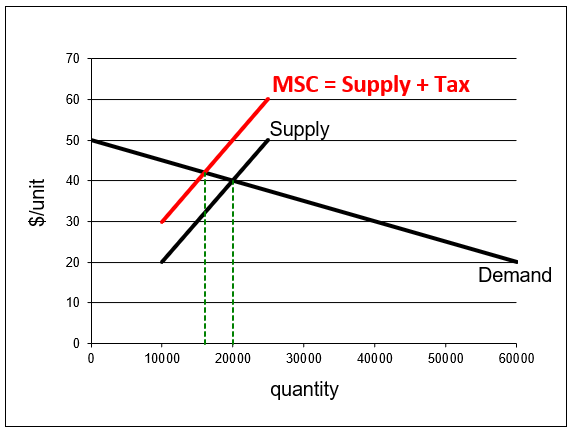
The Pigovian tax shifts the supply curve up so that, if properly calibrated, the amount of the tax reflects the external cost not taken into account. Figure 21.28 shows how a Pigovian tax fixes the market failure caused by externality. Notice that the Supply + Tax curve equals the MSC. This enables the market equilibrium solution to equal the socially optimal solution.
Figure 17.28: Pigovian tax correcting the inefficiency from an externality.
Source: Externality.xls!Externalities.
The Excel workbook Externality.xls enables you to correct the externality with a Pigovian tax.
STEP With an externality in place, click the scroll bar to fix the inefficiency.
With every click, the market supply curve shifts up because you are imposing additional tax. A Pigovian tax works like a regular taxit shifts the supply curve up. Obviously, you want to set the tax so that the black supply curve is coincident with and covers the red MSC curve.
The Pigovian tax fixes the inefficiency caused by the negative externality when the amount of the tax takes the place of the divergence between marginal social and private cost. You know you have the right tax when the market’s equilibrium output equals the socially optimal level of output at 16,000 units.
Unlike regular taxes, which are applied to generate revenue for the government and cause the equilibrium quantity to be less than the optimal quantity, Pigovian taxes are actually applied to correct a market failure. They do generate revenue, but the primary purpose of a Pigovian tax is to change the market’s equilibrium output to allocate resources optimally.
Pigou’s approach dominated economics for many years. Then, in 1960, Ronald Coase (1910 - 2013), who spent most of his long career at the University of Chicago, offered an ingenious alternative: Define property rights over all resources (such as clean air) to internalize the externality. It took some time, but Coase’s approach caught on and would win him the 1991 Nobel award in economics.
In essence, Coase cures the "market failure" by creating more markets. Market failure is in quotation marks because the argument is that it is not a market failure since we do not have complete property rights over all resources. A little intellectual history will help clear this up.
Frank Knight (at the University of Chicago) disagreed with Pigou in an article way back in 1924. Pigou used too much traffic as an example of a market failure in his influential book, The Economics of Welfare, in 1920. On page 194, Pigou explained that individual drivers would fail to take into account the additional congestion they caused when deciding whether to take one road versus another. Thus, the drivers would distribute themselves inefficiently. He pointed out that the government could impose a toll, a tax to use the road, to fix this market failure (Pigou used the phrase laissez-faire and it would not be until the 1950s that "market failure" was coined).
In his 1924 paper, Knight replied that, far from this being a market failure, the problem created by the externality was that there was a missing market! He said Pigou’s logic was error free. It is true that drivers following their own self-interest would produce too much congestion. It is true that this decentralized system failed and a corrective tax would fix it. But, said Knight, while decentralized, this is not a market system because nobody owns the roads. Not all decentralized systems are automatically market systems.
Knight maintained that you cannot blame the market system for a lack of property rights. In Knight’s view, a properly functioning market system would force firms to pay for all of the resources used. A negative externality meant that firms would treat some resources as free and it is no surprise that they would overuse those resources.
Pigou removed the traffic congestion externality example from the next edition of his book. He left, however, the overall framework of corrective taxes and subsidies intact and it became part of the paradigm of economics. For decades, students learned that corrective taxes and subsidies could and should be used to fix inefficient levels of equilibrium output.
In 1960, Coase wrote his most famous article (and perhaps the most often cited article in the history of economics), “The Problem of Social Cost.” He explained how more property rights would enable markets to cure externalities. For a negative spillover like pollution, instead of command and control or a government tax, Coase advocated establishing property rights to clean air and letting the market work its magic. Firms would no longer treat the air as free if they had to pay to use it.
There is no Excel implementation of Coase’s solution. The idea is simply that unpriced resources be priced. This happens when unowned resources are assigned owners. This creates a market, buyers and sellers, for the resource. This directly internalizes the externality.
Coase has said that the property rights solution was influenced by Knight. They were colleagues at the University of Chicago for many years. Knight is known as the father of Chicago School economics and an impact on the work of many social scientists at Chicago and around the world.
A theorem bears Coase’s name and a brief explanation of its content is in order. The Coase Theorem arises out of the idea that more finely delineated property rights enable the market to solve the problem of externality. The word theorem is loosely used here and Coase never claimed to have found or in any sense proved the Coase Theorem.
Coase showed that by settling property rights disputes, courts played a key role in enabling markets to work. Before the court ruled, trade would be impossible because there was disagreement over ownership. These high transactions costs would prevent negotiation.
Once the court ruled, there would be a clear potential buyer and seller. Coase argued that it was not important who won the case because the resource would end up with whoever valued it more. By giving one party the property right, the court established ownership and enabled the resource to be traded. If the winner valued the resource more, the loser would be unwilling to buy it. If the winner valued it less, the loser would buy the resource. Either way, said Coase, once the judge ruled, the resource would end up at its most highly valued use. This idea is now known as the Coase Theorem.
So, in the case of pollution, perhaps homeowners would sue the polluting firm. The court would rule and, either way, once the property right was established, the market would begin to function. Assuming the polluting firm values the property more, it will buy the right to pollute if it loses and will not sell the right if it wins the court case. Either way, it incorporates the cost of pollution because it has to purchase the right if it loses or it recognizes the opportunity cost of having the asset if it wins.
Coase criticized Pigovian taxes and subsidies as a way to fix inefficiency in the allocation of resources by a market system. Coase saw Pigou’s approach as hopelessly idealistic and impossible to implement in the real world. It is easy to draw Figure 17.27 and a snap to show that the correct tax or subsidy enables the market to hit the socially optimal output as in Figure 17.28.
Unfortunately, this blackboard economics (as Coase derisively called it) is easy to draw and teach, but almost impossible to implement. The government regulator will know neither the demand nor the supply functions, and changes over time imply constant tweaking of optimal taxes or subsidies.
Economists think of Coase and Pigou as locking horns and often cast the issue as free market versus regulation. It is clear, however, that Coase and Pigou share some common ground. They both seek to maximize the value of output; they want to optimally allocate resources.
Both offer solutions that work well in theory, but can prove difficult to implement. Once we recognize that neither approach is perfect, we can begin the difficult task of deciding which approach is better in a particular situation.
The EPA and Acid Rain
Although Pigovian taxes remain a staple of economics, in recent years, market-based strategies relying on Coase’s logic have gained popularity.
For example, cap and trade works by creating a total amount of allowable pollution and creating a market where firms can buy and sell rights to pollute. This forces firms to take into account the full costs of their production decisions. They must buy a permit in order to pollute and this forces them to internalize the externality.
The EPA’s sulfur dioxide (SO2) cap and trade program is aimed at decreasing pollutants that cause acid rain, www.epa.gov/airmarkets/allowance-markets. Instead of command and control or taxes, the EPA sets a total emissions constraint, or bubble, then allows firms in the bubble to buy and sell pollution permits. This scheme is equivalent to setting up a market for pollution.
There are many details to be worked out when setting up a market. For example, the government can give each firm an initial allocation of permits or they can auction off the permits.
Some environmentalists remain strongly opposed to market-based solutions to pollution abatement. They see such programs as “licenses to pollute.” But the market’s ability to price resources correctly and enable socially optimal resource allocation is a powerful factor in favor of the market.
Other countries (including such different places as Europe, Costa Rica, and China) have started emissions trading programs. The idea of creating a market for pollution to correct the market failure caused by externality is most definitely a real, practical solution that continues to grow in popularity.
Externalities, Market Failure, and Corrective Action
Externalities are costs or benefits not taken into account by the decision maker. Externalities cause inefficiency because the equilibrium level of output does not equal the socially optimal level of output. As usual, we can measure the inefficiency in the allocation of resources caused by an externality by computing the deadweight loss.
The inefficiency caused by externality can be corrected by command and control, but this approach requires micromanagement by government regulators. Pigovian taxes and subsidies are a type of government regulation that allows individual agents to decide what to do. A firm, for example, would decide how much to pollute and produce, but they have to pay tax. The Pigovian tax is optimized to push the market to the socially optimal output.
The Pigovian approach is definitely at play in the area of education. Truancy laws and other absolute requirements concerning schooling are an example of command and control. Government support of higher education through student grant and loan programs are Pigovian subsidies. The idea is to help students capture the full benefit of a college education and ensure that private decision making is socially optimal.
Another repair relies on market-based solutions to the inefficiency created by externality. Instead of taxing or subsidizing buyers or sellers, property rights for unowned and unpriced resources are established and then the market is left to work its magic. Cap and trade is an example of this approach.
Coase is credited with the idea of fixing inefficient market outcomes with property rights, but Knight definitely had an influence. Knight’s criticism of Pigou’s toll road example is long forgotten, but it contained the seed of the logical argument that a Pigovian market failure is no such thing because not all decentralized systems are market systems.
Mechanism design is a new subfield in economics where we consciously design a game and then let agents play to reach a desired result. This is totally different than the evolution of the market system. Adam Smith did not draw up a blueprint for a market-based society. It happened organically. But now that we know how it works, we are trying to design institutions that give desirable results.
Exercises
Give an example of a positive externality in consumption.
Analyze the welfare effects of a positive externality in consumption. Use Word’s Drawing Tools to support your answer with a demand and supply graph.
In each case that follows, describe the regulatory strategy to correct the market failure caused by a positive externality in consumption.
Command and control
Pigou
Coase
References
The epigraph is from the first page of Eric S. Maskin, “The Invisible Hand and Externalities,” The American Economic Review, Vol. 84, No. 2, Papers and Proceedings of the Hundred and Sixth Annual Meeting of the American Economic Association (May, 1994), pp. 333–337, www.jstor.org/stable/2117854.
“The Problem of Social Cost” was published by Ronald Coase in the fledgling journal of a new field, Journal of Law and Economics, Vol. 3 (October, 1960), pp. 1–44, www.jstor.org/stable/724810.
The transcript of a conversation about Coase’s article and the Chicago School in general is in Edmund W. Kitch, “The Fire of Truth: A Remembrance of Law and Economics at Chicago, 1932–1970,” Journal of Law and Economics, Vol. 26, No. 1 (April, 1983), pp. 163–234, www.jstor.org/stable/725189. George Stigler describes the presentation by Coase to a “collection of superb theorists” as "one of the most exciting intellectual experiences of my life:"
My recollection is that Ronald didn’t persuade us. But he refused to yield to all our erroneous arguments. Milton would hit him from one side, then from another, then from another. Then to our horror, Milton missed him and hit us. At the end of that evening the vote had changed. There were twenty-one votes for Ronald and no votes for Pigou. (p. 221)
That was no typo on Coase’s lifespan in the text, 1910 - 2013. And he worked to the end. In 2009, at the age of 99, he published a book, with Ning Wang, How China Became Capitalist.
Arthur Cecil Pigou’s The Economics of Welfare was first published in 1920 and is freely available online at the Library of Economics and Liberty,
Frank H. Knight’s criticism of Pigou’s traffic congestion example is in “Some Fallacies in the Interpretation of Social Cost,” The Quarterly Journal of Economics, Vol. 38, No. 4 (August, 1924), pp. 582–606,


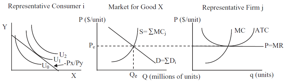 Figure 17.25: An overall view of supply and demand.
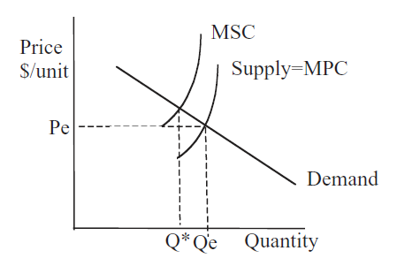 Figure 17.26: A broken market with a negative production externality.
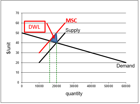
 scroll bar to fix the inefficiency.