2.2: Utility Functions

Previously, we showed that a consumer has preferences that can be revealed and mapped. The next step is to identify a particular functional form, called a utility function, which faithfully represents the person’s preferences. Once you understand how the utility function works, we can combine it with the budget constraint to solve the consumer’s optimization problem.

Cardinal and Ordinal Rankings

Jeremy Bentham (1748-1832) was a utilitarian philosopher who believed that, in theory, the amount of utility from consuming a particular amount of a good could be measured. So, for example, as you ate an apple, we could hook you up to some device that would report the number of “utils” of satisfaction received. The word utils is in quotation marks because they do not actually exist, but Bentham believed they did and would one day be discovered with an advanced measuring instrument. This last part is not so crazyan fMRI machine is exactly what he envisioned.

Bentham also believed that utils were a sort of common currency that enabled them to be compared across individuals. He thought society should maximize aggregate or total utility and utilitarianism has come to be associated with the phrase “the greatest happiness for the greatest number.” Thus, if I get 12 utils from consuming an apple and you get 6, then I should get the apple. Utilitarianism also implies that if I get more utils from punching you in the face than you lose, I should punch you. This is why utilitarianism is not highly regarded today.

This view of utility treats satisfaction as if we could place it on a cardinal scale. This is the usual number line where 8 is twice as much as 4 and the difference between 33 and 30 is the same as that between 210 and 207.

Near the turn of the 20^th century, Vilfredo Pareto (1848-1923, pronounced pa-RAY-toe) created the modern way of thinking about utility. He held that satisfaction could not be placed on a cardinal scale and that you could never compare the utilities of two people. Instead, he argued that utility could be measured only up to an ordinal scale, in which there is higher and lower, but no way to measure the magnitude between two items.

Notice how Pareto’s approach matches exactly the way we assumed that a consumer could choose between bundles of goods as preferring one bundle or being indifferent. We never claimed to be able to measure a certain amount of satisfaction from a particular bundle.

For Pareto, and modern economics, the numerical value from a particular utility function for a given combination of goods has no meaning. These values are like the star ranking system for restaurants.

Suppose Critic A uses a 10-point scale, while Critic B uses a 1000-point scale to judge the same restaurants. We would never say that B’s worst restaurant, which scored say 114, is better than A’s best, a perfect 10. Instead, we compare their rankings. If A and B give the same restaurant the highest ranking (regardless of the score), it is the best restaurant.

Now suppose we are reading a magazine that uses a 5-star rating system. Restaurant X earns 4 stars and Restaurant Y 2 stars. X is better, but can we conclude that X is twice as good as Y? Absolutely not. An ordinal scale is ordered, but the differences between values are not important.

Pareto revolutionized our understanding of utility. He rejected Bentham’s cardinal scale because he did not believe that satisfaction could be measured like body temperature or blood pressure. Pareto showed that we could derive demand curves with the less restrictive more-or-less ranking of bundles.

The transition from Bentham’s cardinal view of utility to Pareto’s ordinal view was not easy. Using the same word, utility, creates confusion (although, to be fair, Pareto tried to create a new word, ophelimity, but it never caught on). It bears repeating that, for a modern economist, although a utility function will show numerical values, these should not be interpreted on a cardinal scale, nor should numerical utilities of different people be compared. Since we cannot make interpersonal utility comparisons to add utilities of different people, we cannot give me the apple or let me punch you.

Monotonic Transformation

Once we reveal the consumer’s indifference curve and map, we have the consumer’s rankings of all possible bundles. Then, all we need to do is use a function that faithfully represents the indifference curves. The utility function is a convenient way to capture the consumer’s ordering.

There are many (in fact, an infinity) of functions that could work. All the function has to do is preserve the consumer’s preference ranking.

A monotonic transformation is a rule applied to a function that changes (transforms) it, but maintains the original order of the outputs of the function for given inputs. Monotonic is a technical term that means always moving in the same direction.

For example, star ratings can be squared and the rankings remain the same. If X is a 4-star and Y a 2-star restaurant, we can square them. X now has 16 stars and Y has 4 stars. X is still higher ranked than Y. In this case, squaring is a monotonic transformation because it has preserved the ordering and X is still higher than Y.

Can we conclude that X is now four times better? Of course not. Remember that the star ranking is an ordinal scale so the distance between items is irrelevant. We say that squaring is a monotonic transformation because it maintains the same ordering and we do not care about the distances between the numeric values. Their only meaning is "higher" and "lower," which indicate better and worse.

It is a fact that the MRS (at any point) remains constant under any monotonic transformation. This is an important property of monotonic transformations that we will illustrate with a concrete example in Excel.

Cobb-Douglas: A Ubiquitous Functional Form

STEP Open the Excel workbook Utility.xls, read the Intro sheet, and then go to the CobbDouglas sheet to see an example of this utility function: \[u(x_1, x_2) = x_1^cx_2^d\]

In economics, a function created by multiplying variables that are raised to powers is called a Cobb-Douglas functional form.

STEP Follow the directions on the sheet (in column K) to rotate the 2D chart so you are looking down at it.

A top-down view of the utility function looks like an indifference map. The utility function itself, in 3D, is a hill or mountain (that keeps growing without ever reaching a topillustrating the idea of insatiability).

With a utility function, the indifference curves appear as contour lines or level curves. The curves in 2D space are created by taking horizontal slices of the 3D surface. Every point on the indifference curve has the exact same height, which is utility.

STEP The exponents (c and d) in the utility function express “likes and dislikes.” Try c = 4 then c = 0.2 in cell B5.

The higher the c exponent, the more the consumer likes \(x_1\) because each unit of \(x_1\) is raised to a higher power as c increases. Notice that when c = 4, the fact that the consumer likes \(x_1\) much more than when c = 0.2 is reflected in the shape of the indifference curve. The steeper the indifference curve, the higher the MRS (in absolute value) and the more the consumer likes \(x_1\).

STEP Proceed to the CobbDouglasLN sheet, which applies a monotonic transformation of the Cobb-Douglas function. It applies the natural log function to the utility function.

Recall that the natural logarithm of a number x is the exponent on e (the irrational number 2.7128 . . .) that makes the result equal x. You should also remember that there are special rules for working with logs. Two especially common rules are \(\ln (x^y) = y \ln x\) and \(\ln (xy) = \ln x + \ln y\). We can apply these rules to the Cobb-Douglas function when we take the natural log:

\(u(x_1, x_2) = x_1^cx_2^d\)

\(\ln [u(x_1, x_2)] = \ln [x_1^cx_2^d]\)

\(\ln [u(x_1, x_2)] = c \ln x_1 + d \ln x_2\)

The CobbDouglasLN sheet applies the natural log transformation by using Excel’s LN() function.

STEP Click on any cell between B12 and Q27 to see the formula. We are computing the natural log of utility, which is \(x_1\) raised to the c power times \(x_2\) raised to the d power.

How does the original utility function compare to its natural log version?

STEP Go back and forth a few times between the two (click on the CobbDouglas sheet tab and then the CobbDouglassLN sheet tab). It is obvious that the numbers are different.

But did you notice something curious?

STEP Compare the cells with yellow backgrounds in the two sheets to see that these two combinations continue to lie on the same indifference curve, even though the utility values of the two functions are different.

The fact that the cells remain on the same indifference curve after undergoing the natural log transformation demonstrates the meaning of a monotonic transformation. The utility values are different, but the ranking has been preserved. The two utility functions both maintain the same relationship between 1,14 and 2,7 and every other bundle.

So now you know that a Cobb-Douglas utility function can be used to faithfully represent a consumer’s preferences (including tweaking the c and d exponents to make the curves steeper or flatter) and that we can use the natural log transformation if we wish. In addition, economists often use the Cobb-Douglas functional form for utility (and production) functions because it has very nice algebraic properties where lots of terms cancel out.

The Cobb-Douglas function is especially easy to work with if you remember the following rules:

Algebra Rules: \(\frac{x^a}{x^b} = x^{a - b}\) and \(x^{a^b} = x^{ab}\)

Calculus Rule: \(\frac{dax^b}{dx} = bax^{b - 1}dx\)

These rules may seem irrelevant right now, but we will see that they make the Cobb-Douglas function much easier to work with than other functions. This goes a long way in explaining the repeated use of the Cobb-Douglas functional form in economics.

Expressing Other Preferences with Utility Functions

STEP Proceed to the PerfSub sheet and look around. Scroll down (if needed) and look at the two charts.

Notice how this functional form is producing straight line indifference curves (in the 2D chart). If the consumer treated two goods as perfect substitutes, we would use this functional form instead of Cobb-Douglas. The coefficients (a and b) can be tweaked to make the lines steeper or flatter.

STEP Proceed to the PerfComp sheet. This shows how the min() functional form produces L-shaped indifference curves.

The min() function outputs the smaller of the two terms, \(ax_1\) and \(bx_2\). This means that getting more of one good while holding the amount of the other good constant does not increase utility. This produces an L-shaped indifference curve.

Finally, the Quasilinear sheet displays indifference curves that are actually curved, but rather flat.

STEP Go to the Quasilinear sheet and click on the different functional form options. These are just a few of the many transformations that can be applied to \(x_1\) and then added to \(x_2\) to produce what is called quasilinear utility. Later, we will see that this functional form has different properties than Cobb-Douglas.

Note that we can represent many different kinds of preferences with utility functions. An important point is that there are many (to be more exact, an infinity) of possible utility functions available to us. We would choose one that faithfully reflects a particular consumer’s preferences. We can always apply a monotonic transformation and it will not alter the consumer’s preferences.

Computing the MRS for a Utility Function

Now that we have utility functions to represent a consumer’s preferences, we are able to compute the MRS from one point to another (like we did in the previous chapter) or by using the instantaneous rate of change, better known as the derivative.

This is not a mathematics book, but economists use math so we need to see exactly how the derivative works. The core idea is convergence: make the change in x (the run) smaller and smaller and the ratio of the rise over the run (the slope) gets closer and closer to its ultimate value. The derivative is a shortcut that gives us the answer without the cumbersome process of making the change smaller and smaller.

But this is way too abstract. We can see it in Excel.

STEP Proceed to the MRS sheet to see how the MRS can be computed via a discrete-size change versus an infinitesimally-small change.

The utility function is \(x_1x_2\). This is Cobb-Douglas with exponents (implicitly) equal to 1.

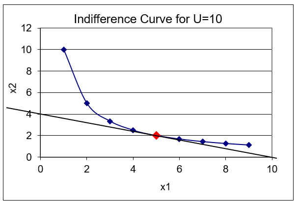
Suppose we are interested in the indifference curve that gives all combinations with a utility of 10. Certainly 5,2 works (since 5 times 2 is 10). It is the red dot in the graph on the MRS sheet (and in Figure 2.10).

Figure 10: Computing the MRS.

Source: Utility.xls!MRS

From the bundle 5,2, if we gave this consumer 1 more unit of \(x_1\), by how much would we have to decrease \(x_2\) to stay on the \(U=10\) indifference curve? A little algebra tells us.

We know that \(U = x_1x_2\) and the initial bundle 5,2 yields \(U = 10\). We want to maintain U constant with \(x_1 = 6\) because we added one unit to \(x_1\), so we have:

\(U = x_1x_2\)

\(10 = 6x_2\)

\(x_2 = \frac{10}{6}\)

We have two bundles that yield \(U = 10\) (5,2, and 6,\(\frac{10}{6}\)). We can compute the MRS as the change in \(x_2\) divided by the change in \(x_1\). The delta (or difference) in \(x_2\) is \(-\frac{1}{3}\) (because \(\frac{10}{6}\) is \(\frac{1}{3}\) less than 2) and the delta in \(x_1\) is 1 (6 - 5), so starting from the point 5,2, the MRS from \(x_1\) = 5 to \(x_1\) = 6 is \(-\frac{1}{3}\). This is what Excel shows in cell C18.

Another way to compute the MRS uses the calculus approach. Instead of a “large” or discrete-size change in \(x_1\), we take an infinitesimally small change, computing the slope of the indifference curve not from one point to another, but as the slope of the tangent line (as shown in Figure 2.10). We use the derivative to compute the MRS at a particular point.

For this simple utility function, holding U constant at 10, we can rewrite the function as \(x_2\) in terms of \(x_1\), then take the derivative.

\(U = x_1x_2\)

\(x_2 = \frac{10}{x_1}\)

\(\frac{dx_2}{dx_1} = - \frac{10}{x_1^2}\)

At \(x_1 = 5\), substitute in this value and the MRS at that point is \(-\frac{10}{25}\) or -0.4. This is what Excel shows in cell D18. If you need help with derivatives, the next chapter has an appendix that reviews basic calculus.

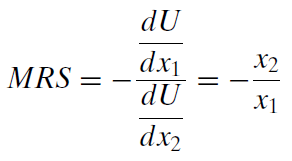
Computing the MRS this way relies on the ability to write \(x_2\) in terms of \(x_1\). If we have a utility function that cannot be easily rearranged in this way, we will not be able to compute the MRS. There is, however, a more general approach. The procedure involves taking the derivative of the utility function with respect to \(x_1\) (called the marginal utility of \(x_1\)) and dividing by the derivative of the utility function with respect to \(x_2\) (called the marginal utility of \(x_2\)). Do not forget to include the minus sign when you use this approach. Here is how it works.

With \(U = x_1x_2\), the derivatives are simple: \(\frac{dU}{dx_1} = x_2\) and \(\frac{dU}{dx_2} = x_1\). Thus, we can substitute these into the numerator and denominator of the MRS expression:

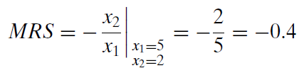
Because we are considering the point 5,2, we evaluate the MRS at that point (which means we plug in those values to our MRS expression), like this:

Note that minus the ratio of the marginal utilities gives the same answer as the \(\frac{dx_2}{dx_1}\) method. Both are using infinitesimally small changes to compute the instantaneous rate of change of the indifference curve at a particular point.

Also note that the ratio of the marginal utilities approach requires that you divide the marginal utility of \(x_1\) (the good on the x axis) by the marginal utility of \(x_2\) (the good on the y axis). Since we used \(\frac{\Delta y}{\Delta x}\) in the discrete-size change approach, it is easy to confuse the numerator and denominator when computing the MRS via the derivative. Remember that \(\frac{dU}{dx_1}\) goes in the numerator.

Comparing \(\Delta\) and d Methods

So far, we know there are two ways to get the MRS: move from one point to another along the indifference curve (discrete change, \(\Delta\)) or slope of the tangent line at a point (infinitesimally small change, d). We also know that we have two ways of doing the latter (solve for \(x_2\) then take the derivative or compute the ratio of the marginal utilities.)

But you may have noticed a potential problem in that the two procedures to get the MRS yield different answers. In the MRS sheet and our work above, the discrete change approach tells us that the MRS as measured from \(x_1 = 5\) to \(x_1 = 6\) is \(-\frac{1}{3}\), whereas the derivative method says that the MRS at \(x_1 = 5\) is -0.4.

This difference in measured MRS is due to the fact that the two approaches are applying a different size change in \(x_1\) to a curve. As the discrete-size change gets smaller, it approaches the derivative measure of the MRS. You can see this clearly with Excel.

STEP Change the step size in cell B7 to 0.5 and watch how cell C18 changes. Notice that the chart is also slightly different because the point at \(x_1 = 6\) is now at 5.5.

You have made the size of the change in \(x_1\) smaller so the point is now closer to the initial value, 5.

STEP Do it again, this time changing the step size in cell B7 to 0.1. The point with \(x_1 = 5.1\) is so close to 5 that it is hard to see, but it is there. Do one last change to the step size, setting it at 0.01.

With the step size at 0.01, you cannot see the initial and new points because they are so close together, but they are still a discrete distance apart. Excel displays the point-to-point delta computation in cell C18. It is really close to the derivative measure of the MRS in cell D18 because the derivative is simply the culmination of this process of making the change in \(x_1\) smaller and smaller.

In Figure 2.10, the discrete change approach is computing the rise over the run using two separate points on the curve, while the calculus approach is computing the slope of the tangent line.

STEP Look at the values of the cells in the yellow highlighted row.

The MRS for a given approach are exactly the same. In other words, columns C, H, and M are the same and columns D, I, and N are the same. This shows that the MRS remains unaffected when the utility function is monotonically transformed.

Utility Functions Represent Preferences

Utility functions are equations that represent a consumer’s preferences. The idea is that we reveal preferences by having the consumer compare bundles, and then we select a functional form that faithfully reflects the indifference curves of the consumer.

In selecting the functional form, there are many possibilities and economists often use the Cobb-Douglas form. The values of utility produced by inputting amounts of goods are meaningless and any monotonic transformation (because it preserves the preference ordering) will work as a utility function. Monotonic transformations do not affect the MRS.

The MRS is an important concept in consumer theory. It tells us the willingness to trade one good for another and this measure the consumer’s likes and dislikes. Willingness to trade a lot of y for a little x produces a high MRS (in absolute value) and this indicates that the consumer values x more than y.

The MRS computed from one point to another (\(\Delta\)), but it can also be computed using the derivative (d) at a point. Both are valid and the resulting number for the MRS is interpreted the same way (willingness to trade).

Exercises

The utility function, \(U = x - 0.03x^2 + y\), has a quasilinear functional form. Use this function to the answer the questions below. You can see what it looks like by choosing the Polynomial option in the Quasilinear sheet.

1. Compute the value of the utility function at bundle A, where x = 10 and y = 1. Show your work.
2. Working with bundle A, find the MRS as x rises from x = 10 to x = 20. Show your work.
3. Find the MRS at the point 10,1 (using derivatives). Show your work.
4. Why do the two methods of determining the MRS yield different answers?
5. Which method is better? Why?

References

The epigraph can be found on page 91 of the revised edition of The Foundations of Economic Analysis, by Paul Samuelson. This remarkable book, written by one of the greatest economists of the 20^th century, took economics to a new level of mathematical sophistication. Samuelson could not have picked a better opening quote, “Mathematics is a Language,” by J. Willard Gibbs.