Without a doubt, the demand curve is the most important idea in the Theory of Consumer Behavior. We have derived the demand curve analytically and numerically. The demand curve tells us the optimal amount to buy at a given price. It also tells us how quantity demanded will change as price changes, ceteris paribus.
This section remains focused on the demand curve, extending the analysis of the consumer’s optimal response to a change in price. The core concept is that the total effect on quantity demanded (given by the demand curve) for a given change in price can be broken down into two separate effects, called income and substitution effects.
Our attention is still on the change in quantity demanded as price changes, ceteris paribus, but by breaking apart the observed response when price changes, we get a deeper explanation of demand. We also explain how we might get a Giffen good.
Intuition
Before diving into complicated graphs and math, let’s review the story behind income and substitution effects. Seeing the big picture improves your chances of really understanding what income and substitution effects are all about.
Suppose that, ceteris paribus, price rises. We know the consumer has to re-optimize. We know the consumer will choose a new optimal combination of goods. We can see the consumer buy a different amount after the price changes. If we simply compute the change in the amount purchased of \(x_1\) before and after the price change, we are comparing two points on the demand curve. This is called the total effect of a price change.
The breakthrough idea is that the increase in price has two channels by which it affects the consumer. One channel focuses on the fact that a price increase is like a decrease in purchasing power. After all, given an income level, if prices double, then I can buy half of what I bought before. My income has not changed, but my purchasing power has fallen just the same as if my income had been cut in half. The income effect reflects the fact that price changes affect optimal quantity demanded by altering purchasing power.
The other channel is called the substitution effect. The idea is that a price change in one good alters the relative prices faced by the consumer and induces substitution of the relatively cheaper good for the relatively more expensive one. When \(p_1\) rises, \(x_1\) is relatively more expensive than \(x_2\) and so I am naturally going to avoid \(x_1\) and be attracted to \(x_2\).
Figure 4.17 shows the two channels below the total effectthey are submerged and not directly observed. Added together, they make up the total effect.
Figure 4.17: The basic idea behind income and substitution effects.
We will see that the income effect can be either positive or negative, but the substitution effect is always negative (assuming well-behaved preferences). When price goes up, the substitution effect says "buy less." Of course, if price falls, the reverse occurs and, according to the substitution effect alone, consumption increases.
The reason the income effect is ambiguous in sign is the fact that there are normal and inferior goods. If the good is normal, then optimal \(x_1\) rises as income increases, but if the good is inferior, then consumption and income are inversely related.
Finally, it helps to know the underlying motivation behind the discovery of income and substitution effects. Economists were arguing about the existence of Giffen goods. The Law of Demand said price and quantity were inversely related. Income and substitution effects explained under which conditions Giffen behavior (an upward sloping demand curve) is possible. We will see that if the income and substitution effects work together, then the demand curve is guaranteed to be downward sloping. Understanding income and substitution effects will allow us to give a more refined, precise definition of the Law of Demand.
Numerical Example of Income and Substitution Effects
STEP Open the Excel workbook IncSubEffects.xls, read the Intro sheet, and proceed to the OptimalChoice sheet.
We have the usual Cobb-Douglas utility function with a conventional budget line. We have done this problem before and the initial optimal solution is 25,\(16 \frac{2}{3}\).
STEP Decrease \(p_1\) by 1 to $1/unit (in cell B17).
Figure 4.18 displays what is on your screen. The red line is the familiar new budget line (after the price decrease). There is, however, a dashed line that has not been used before. This dashed line represents the outcome of a thought experiment.
Figure 4.18: Decreasing \(p_1\).
Source: IncSubEffects.xls!OptimalChoice
STEP Click the button to see a second graph of the situation. It has the axes scale adjusted so you can see better what is going on.
The dashed line is critical to understanding the splitting of the total effect into income and substitution effects. It has the same slope as the new budget line, yet it goes through the initial optimal solution. What we have done is pretend to take away enough income from the consumer to enable him to buy the initial bundle with the new, lower \(p_1\).
We took away income (shifting down the budget constraint relative to the new budget line) because the fall in price implies an increase in purchasing power. Had there been a price rise, we would have had to increase income to compensate for the price increase.
We will find a tangency solution on the dashed line and this will allow us to split the total effect into the income and substitution effects.
Of course, nothing like this actually happens in the real world. When the price falls, the consumer re-optimizes, buying a new optimal bundle, and that is the end of the story. But for the purposes of understanding the demand curve, we figure out what the consumer would buy at the imaginary dashed line and we use that to split the total effect into the substitution and income effects.
But this is all way too abstract. Let’s actually do it so you can see how it works. To figure out how much income to take away to cancel out the changed purchasing power from the price change, we use the Income Adjuster Equation. \[\Delta m = x_1 \mbox{*}\Delta p_1\] Applied to this problem, we know that \(x_1 \mbox{*}\) is 25 (from the initial optimal solution) and the change in \(p_1\) is \(-1\) (because the price fell from 2 to 1, so \(new - initial\) is \(1 - 2\)); thus, we have: \[\Delta m = x_1 \mbox{*}\Delta p_1\] \[\Delta m = [25][-1] = -25\] The minus tells us that we have to take away income. The dashed line is based on an income of $75, \(p_1 = 1\), and \(p_2 = 3\).
In summary, we have three budget lines when we work with income and substitution effects: (1) the usual initial line, (2) the usual new line from the change in price, and (3) the imaginary (dashed) line that has been adjusted to pass through the initial optimal solution.
We find the usual new optimal solution so we can compute the total effect first, then we use the dashed line to find the income and substitution effects.
STEP With \(p_1 = 1\), run Solver.
Figure 4.19 shows that the consumer chooses the 50,\(16 \frac{2}{3}\) combination. Thus, we have two points to consider so far:
Point A: Initial: At \(m = 100, p_1 = 2, x_1 \mbox{*} = 25, x_1 \mbox{*} = 16 \frac{2}{3}\).
Point C: New: At \(m = 100, p_1 = 1, x_1 \mbox{*} = 50, x_1 \mbox{*} = 16 \frac{2}{3}\).
Figure 4.19: New optimal solution at \(p_1 = 1\).
Source: IncSubEffects.xls!OptimalChoice
Notice that Excel displays three difference curves around the current optimal solution, but there are actually an infinite number of curves going through every point in the quadrant. With \(c = d = 1\) being held constant, the indifference map is not changing in any way. We are simply displaying different indifference curves whenever \(x_1\) and \(x_2\) in cells B12 and B13 change.
Points A and C are two points on the price consumption curve and two points on the demand curve. The total effect of a $1/unit decrease in the price of good 1 can be found by measuring the movement from A to C: for \(x_1\), the total effect is \(+25\) units and for \(x_2\), the total effect is zero (\(x_2 \mbox{*} = 16 \frac{2}{3}\) before and after the price shock).
The total effect can be directly observed. With the initial price, we can see the consumer purchase 25 units of good 1 and \(16 \frac{2}{3}\) of good 2. We see the price of good 1 fall by $1/unit and watch the consumer respond by buying 25 units more of \(x_1\) and leaving the amount of \(x_2\) unchanged.
We are now ready for the key move. We will hypothetically take away exactly $25 of income so we can find the optimal solution on the imaginary, dashed line. The consumer does not actually have income taken away. It is a thought experiment. Working out what the consumer would do in this hypothetical situation allows us to split the total effect into its constituent parts.
STEP Change income to $75 (notice that the budget line now lies on top of the dashed budget line) and run Solver.
You can safely ignore the steeper line in the chartall we want is point B, the optimal solution with the dashed budget line. Solver tells us that point B is 37.5,12.5. This gives us three points to consider:
Point A: Initial: At \(m = 100, p_1 = 2, x_1 \mbox{*} = 25, x_2 \mbox{*} = 16 \frac{2}{3}\).
Point B: Unobserved: At \(m = 75, p_1 = 1, x_1 \mbox{*} = 37 \frac{1}{2}, x_2 \mbox{*} = 12 \frac{1}{2}\).
Point C: New: At \(m = 100, p_1 = 1, x_1 \mbox{*} = 50, x_2 \mbox{*} = 16 \frac{2}{3}\).
Look carefully at the three points and concentrate on how points B and C differ: C uses new \(p_1\) with original m, while B is based on new \(p_1\) with adjusted m (adjusted in a special way so that the dashed line goes through point A).
With these three points, we can compute total, income, and substitution effects for \(x_1\) and \(x_2\). The three effects are shown by arrows on the axes of Figure 4.20. This is a complicated graph. Take your time and read it with care. Try to separate the different elements and lines to different parts of the problem: initial (A), new (C), and intermediate positions (B).
Figure 4.20: Total (TE), income (IE), and substitution (SE) effects.
There are effects measured from one point to another for both \(x_1\) and \(x_2\). These \(\Delta\)s are calculated the usual way as \(new - initial\). For \(x_1\), we find:
SE: A to B: \(37 \frac{1}{2} - 25 = 12 \frac{1}{2}\)
IE: B to C: \(50 - 37 \frac{1}{2} = 12 \frac{1}{2}\)
TE: A to C: \(50 - 25 = 25\)
Notice that the total effect (TE) can be found by computing the difference from A to C (\(50 - 25 = 25\)) or taking advantage of the fact that SE + IE = TE, so \(12.5 + 12.5 = 25\). The effects for \(x_1\) are all computed along the x axis in terms of units of \(x_1\).
Analyzing the effect on \(x_2\) of a change in \(p_1\) gives us cross income and substitution effects for \(x_2\), which are shown by arrows on the y axis, in Figure 4.20.
SE: A to B: \(12 \frac{1}{2} - 16 \frac{2}{3} = - 4 \frac{1}{6}\)
IE: B to C: \(16 \frac{2}{3} - 12 \frac{1}{2} = 4 \frac{1}{6}\)
TE: A to C: \(16 \frac{2}{3} - 16 \frac{2}{3} = 0\)
On \(x_2\), the income and substitution effects work against each other. The substitution effect, from A to B, lowers the amount of \(x_2\) since \(p_1\) fell, making \(x_2\) more expensive relative to \(x_1\). But when we move from B to C, the income effect exactly cancels out the SE. The fall in \(p_1\) has increased our purchasing power and, since \(x_2\) is a normal good, we want to buy more of it.
It is a property of the Cobb-Douglas utility function that the cross IE and SE effects cancel each other out, leaving a zero total effect. This is not a usual or common result and it demonstrates how the functional form imposes structure on the demand curve.
Let’s return now to \(x_1\) and focus on its substitution effect, which we know is always negative. This leads immediately to a question: If the SE is always negative, then why is it \(+12.5\) in Figure 4.20?
The answer to this apparent contradiction is that the negative refers to the relationship, not the actual value of the SE. Given that price fell, an increase in quantity purchased is consistent with a negative effect because it is the relationship between the two variables that is being described as negative.
Likewise, the sign of the income effect can be tricky. The key is to pay attention to which shock variable is being considered. The income effect measured as the response to a change in income is positive, in this case, because as I move from B to C, my income is increased and I respond by increasing my optimal consumption of good 1.
Now you might ask, "If the two effects work together, then how is the substitution effect negative and the income effect positive?" This is because we defined the income effect as the response to a change in income, like the movement from point B to C in Figure 4.20. But, if you remember, this example began with a decrease in the price of good 1. The decrease in the price of good 1 can be interpreted as an increase in income, in the sense of greater purchasing power. If we tie the 12.5 increase in good 1 from the income effect to the decrease in price of good 1, we see that this negative relationship reinforces the negative substitution effect and gives a negative total effect.
Now that we know how the income and substitution effects combine to form the total effect of a price change, we can show how easy it is to compute them from a reduced form solution.
We first have to solve the model analytically and get a reduced form expression as a function of \(m\) and \(p_1\). We have done this before for a Cobb-Douglas utility function and found \[x_1 \mbox{*} = (\frac{c}{c+d})\frac{m}{p_1}\] If we substitute in \(c=d=1\), we have \[x_1 \mbox{*} = \frac{m}{2p_1}\] At \(m=100\) and \(p_1=2\), \(x_1 \mbox{*}=25\). This is the initial solution (point A).
If \(p_1\) falls to $1/unit, then we plug in \(m=100\) and \(p_1=1\), which gives the new solution (point C), \(x_1 \mbox{*}=50\). The total effect is \(50 - 25 = 25\).
To find the SE, we need point B. We use the reduced form expression to compute quantity demanded with adjusted m ($75) and new \(p_1\) ($1/unit). \[x_1 \mbox{*} = \frac{m}{2p_1} = \frac{[75]}{2[1]} = 37.5\] Once we have point B, we have split the total effect from A to C and we can compute the SE and IE by going from A to B and B to C, respectively. The SE is \(37.5 - 25 = 12.5\) and the IE is \(50 - 37.5 = 12.5\). These results agree with our earlier work.
Income and Substitution Effects via Graphs
Income and substitution effects are complicated. Figure 4.20 is not easy to understand. There are three budget lines and a lot going on. So what is so important about income and substitution effects that makes it worthwhile to master them?
Income and substitution effects hold the key to explaining how we can get a Giffen good. They mark real progress in economics, settling a long debate about whether or not upward sloping demand curves are possible. We will deconstruct the income and substitution effect graph (Figure 4.20), examining each layer one at a time, to show the source of Giffen behavior.
We begin with Figure 4.21. On the left we have the initial optimal solution and the right displays a single point on the demand curve (not shown).
Figure 4.21: The initial solution.
Next, we decrease the price of good 1, as shown in Figure 4.22, which creates a new budget line. We know the consumer will re-optimize and choose a new optimal solution along the new, flatter line, but Figure 4.22 does not show this new solution quite yet. Instead, it shows the point B solution on a dashed line with the income that would have to be taken away to cancel out the increased purchasing power from the price decrease.
Figure 4.22: A \(p_1\) decrease and imaginary budget constraint.
Figure 4.22 shows the optimal solution, point B, for the hypothetical situation with lower \(p_1\) and adjusted m. The rightward pointing arrow is the SE for \(x_1\) is the substitution effect, from point A to B on the x axis. The dashed line has a flatter slope (new \(p_1\) is less than initial \(p_1\)) through point A. This guarantees that B is to the right of A. This is why the SE is always negative.
It is impossible to draw a point B to the left of A without making the indifference curves cross. With MRS = \(\frac{p_1}{p_2}\) at A, lowering \(p_1\) and adjusting m so dashed line goes through A, means the consumer must move southeast to find the highest indifference curve tangent to the dashed line.
Now, we are ready to show point C. We have a known negative substitution effect and all that remains to be done is to find the indifference curve tangent to the new budget line (with lower \(p_1\)). The key insight is that there are several possible positions for point C. Figure 4.23 shows three possibilities.
Figure 4.23: Understanding Giffen behavior.
Figure 4.23 shows that the final position of point C depends on whether the good is normal or inferior, with a subcategory of inferior goods that are Giffen.
C1: Good 1 is a normal good so the income effect from B to C works together with the movement from A to B and we end up at point C1. In this case, and for any point C to the right of B, we get a downward sloping demand curve.
Good 1 is an inferior good so the income and substitution effects work against each other. The movement from B to C will be to the left and leave us with a point C to the left of B. There are two possibilities:
C2: The income effect pushes the consumer to buy less \(x_1\), but it is less than the substitution effect (which leads to buying more \(x_1\) as \(p_1\) falls). We end up at point C2 between A and B and the demand curve is still downward sloping.
C3: The income effect not only works against the substitution effect, it is stronger, swamping it. Point B to C moves in the opposite direction than A to B and and is bigger than A to B. This leaves the consumer to the left of B at point C3. The demand curve is upward sloping. This is a Giffen good.
It can be difficult to draw a Giffen good correctly because the indifference curves cannot cross. So, in Figure 4.23, the space available for point C3 is tightC3 can only fit to the left of A and to the right of the indifference curve that is shown tangent to B.
Figure 4.23 also makes clear that it is the indifference curves, which come from the utility function, that determine how quantity demanded responds to a change in price. How a good generates utility (i.e., whether utility is Cobb-Douglas, quasilinear, perfect complements, or another functional form) determines whether it is normal, inferior, or Giffen.
The decomposition of the total effect into income and substitution effects provides the condition which must hold for Giffen behavior: the income effect must work against the substitution effect and be bigger. We can reinforce this key insight with a mathematical expression that gives more detail on exactly how we get Giffenness.
The Slutsky Equation
In 1915, decades after the supposed spotting of a Giffen good during the Irish potato famine, Eugen Slutsky published a paper in an Italian journal that showed how to decompose the total effect of a price change into income and substitution effects. He had a mathematical expression that showed how it was possible to get an upward sloping demand curve!
Unfortunately, his work went unnoticed. Twenty years later, John R. Hicks (a Nobel laureate in 1972) and R. G. D. Allen rediscovered the ideas in Slutsky’s paper. Sometimes, the idea of income and substitution effects are referred to as Slutsky-Hicks or Slutsky-Hicks-Allen. We will keep it simple and call it the Slutsky Equation.
The Slutsky Equation, which we will not derive, says in mathematical terms something that we already know: The total effect of a price change can be expressed as the sum of a substitution and an income effect. It turns out that there are several ways to express the decomposition with a Slutsky Equation. Here are two versions: \[\frac{\Delta x_1}{\Delta p_1}=\frac{\Delta x_1^{SE}}{\Delta p_1}+\frac{\Delta x_1^{IE}}{\Delta p_1}\] \[\frac{\Delta x_1}{\Delta p_1}=\frac{\Delta x_1^{SE}}{\Delta p_1}-x_1 \mbox{*}\frac{\Delta x_1}{\Delta m}\] Both equations say the same thing: the total effect, \(\frac{\Delta x_1}{\Delta p_1}\), is equal to the substitution effect, \(\frac{\Delta x_1^{SE}}{\Delta p_1}\), plus the income effect. Where they differ is how they express the income effect.
Look carefully at the denominators. The income effect in the first equation has a \(\Delta p_1\) denominator, like the other two terms. What Slutsky figured out was that the income effect of price change, \(\frac{\Delta x_1^{IE}}{\Delta p_1}\), could be written as \(-x_1 \mbox{*}\frac{\Delta x_1}{\Delta m}\). In other words, the income effect channel of the price change can be expressed as the amount of good 1 initially purchased times the change in \(x_1\) as income changes (the slope of the Engel curve). Notice the minus sign, which picks up the fact that when price falls, that is like an increase in income.
Now we can really see how to get a Giffen good, which has an upward sloping demand curve so \(\frac{\Delta x_1}{\Delta p_1} > 0\). Since the first term, the substitution effect is always negative, we definitely need an inferior good so that \(\frac{\Delta x_1}{\Delta m} < 0\) so that the second term is positive. Obviously, if the good is extremely inferior, so that \(\frac{\Delta x_1}{\Delta m}\) is much less than zero, we might get a Giffen good.
But the Slutsky Equation reveals another way to get Giffen behavior. A large opposing income effect can be obtained by the good being inferior and the consumer buying a lot of it so that \(-x_1 \mbox{*}\frac{\Delta x_1}{\Delta m}\) is a big positive number to outweigh the negative substitution effect. If the good is merely inferior, but the consumer buys little of it, then it less likely to be Giffen.
This is why we look for Giffen behavior in staples, basic commodities that comprise a large share of the budget. Potatoes for the Irish, rice for Asians, and tortillas for Mexicans are three examples that economists have examined for Giffen behavior. For a poor person, these items could be consumed in large quantities, yet, as income rises, quantity demanded falls so they are inferior goods. The combination of a large \(x_1 \mbox{*}\) and \(\frac{\Delta x_1}{\Delta m} < 0\) could produce a large, positive \(-x_1 \mbox{*}\frac{\Delta x_1}{\Delta m}\) term that is bigger than the negative substitution effect.
Remember how we generated Giffen behavior with GiffenGoods.xls in the previous section? We increased the price from $1/unit to $1.1/unit and optimal \(x_1\) rose from 44 to 48.6, while optimal \(x_2\) fell dramatically from 11 to around 1.5. Notice how \(x_1\) is a staple, dominating the amounts purchased of the two goods.
We know its Giffen, but is \(x_1\) also inferior? Let’s find out.
STEP Open GiffenGoods.xls and proceed to the Optimal1 sheet. Click the button and run Solver to make sure you are at the optimal initial solution of 44,11. Increase m to 60 and run Solver. What happens?
Yes, as we know must be true (since we know \(x_1\) is a Giffen good), \(x_1\) is an inferior good: optimal \(x_1\) fell (to 39) as income increased to $60. Giffenness requires that \(x_1\) be inferior and this example also reflects the fact that concentration of the consumer’s budget on an inferior good contributes to the production of a Giffen response.
The Biblio sheet in GiffenGoods.xls, from the previous section, had several references to papers trying to find Giffen goods, yet the jury is still out. What is unquestioned, however, is the theoretical requirement: it must be an inferior good so that the IE is in the opposite direction and larger than the SE.
The Slutsky Equation also enables us to fine tune a statement that is, strictly speaking, false. Introductory economics students around the world learn the Law of Demand: when price increases, ceteris paribus, quantity demanded must fall. In other words, holding everything else constant, quantity demanded and price are inversely related and demand is always downward sloping.
This is fine, at the introductory level, where we do not want to confuse beginning students, but we know that an upward sloping demand curve is possibleit is called a Giffen good. They are a violation of the "Law" of Demand and we know they could exist. When their price rises, so does quantity demanded.
Can we rehabilitate the Law of Demand so there is no exception? Yes, we can. Our knowledge of income and substitution effects points the way. We can more precisely define the Law of Demand. By inserting a qualifying clause, we can get the Law of Demand to be exactly right: If the good is normal, then quantity demanded falls as price rises, ceteris paribus. That is guaranteed to be true because a normal good has an income effect that works together with the substitution effect. Thus, there is no way to get Giffenness.
The Cobb-Douglas utility function cannot give Giffen behavior. The reduced form solution, \(x_1 \mbox{*} = (\frac{c}{c+d})\frac{m}{p_1}\), means that \(\frac{dx_1 \mbox{*}}{dm} = (\frac{c}{c+d})\frac{1}{p_1} > 0\) so the income effect, \(- x_1 \mbox{*}\frac{dx_1 \mbox{*}}{dm}\), is negative. This means the IE and SE are both negative and work together so there is no way the Cobb-Douglas utility function can generate Giffenness.
TE = SE + IE
Income and substitution effects are used by economists to better understand the demand curve and to explain Giffen behavior. By disassembling the total effect of a price change, the Slutsky Equation shows how a Giffen good can arise if the income effect opposes and swamps the substitution effect (which generates an upward sloping relationship between price and quantity demanded).
Given a utility function and budget constraint, we find the initial optimal solution (point A). A price change will lead to a new optimal solution (point C) which we can use to compute the total effect. We can then use the Income Adjuster Equation to find a hypothetical point B that splits the total effect into substitution and income effects.
Given a reduced form expression of \(x \mbox{*} = f(p,m)\), we can find points A, B, and C by evaluating the expression at the appropriate p and m values to compute points A, B, and C.
The Slutsky Equation is a mathematical presentation of income and substitution effects. The math gives us the insight that the income effect, \(-x_1 \mbox{*}\frac{\Delta x_1}{\Delta m}\), is composed of initial optimal \(x_1\) times the response of \(x_1\) to an income change. This reveals that Giffenness is more likely to be found in inferior goods that also attract a high concentration of the consumer’s budget.
There are even more ways to express the Slutsky Equation than the two used in this section. Instead of altering income to allow the consumer to buy the initial bundle of goods, you can change income to allow the consumer to be on the initial indifference curve. This is sometimes referred to as the Hicks substitution effect.
Exercises
Reproduce, using Word’s Drawing Tools, Figures 4.21, 4.22, and 4.23, explaining each graph in your own words.
Repeat question 1, with one key change: apply a price increase in good 1 (instead of a price decrease).
In stating the Law of Demand, some economists choose to include a condition that the good is normal, like this: If the good is a normal good, then price and quantity demanded are inversely related, ceteris paribus. Why is the normal good clause needed?
Given the demand function, \(x_1 \mbox{*} = 20 + \frac{m}{20p_1}\), compute the total, income, and substitution effects when price falls from $5 to $4/unit, with income of $1000. Show your work.
Use the Optimal1 sheet in GiffenGoods.xls to find points A, B, and C for a shock in \(p_1\) from $1 to $1.1/unit. Compute the TE, SE, and IE for \(x 1\). Show your work and explain what you did.
References
The epigraph is from the biography of Slutsky available at the New School’s History of Economic Thought website, www.hetwebsite.net/het/. The site was created and is maintained by Gonçalo L. Fonseca. There are sketches of hundreds of economists, links to other resources, and descriptions of various schools of thought in economics. The intellectual history of economics is fascinating and this website is a wonderful place to browse.


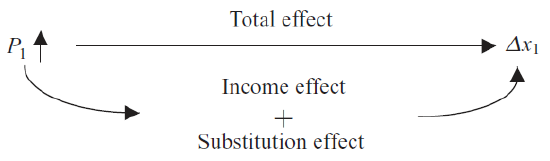 Figure 4.17: The basic idea behind income and substitution effects.
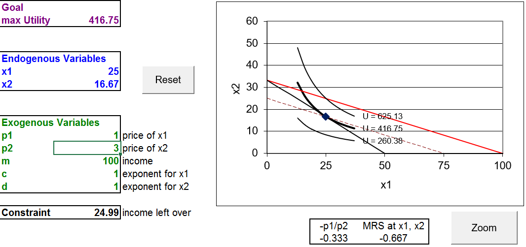
 button to see a second graph of the situation. It has the axes scale adjusted so you can see better what is going on.
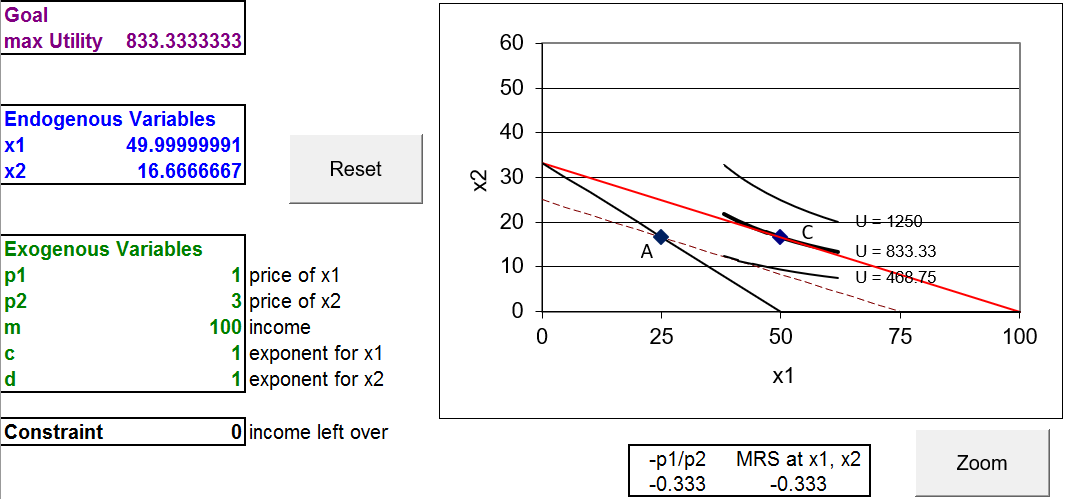
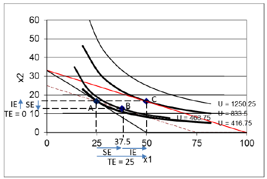 Figure 4.20: Total (TE), income (IE), and substitution (SE) effects.
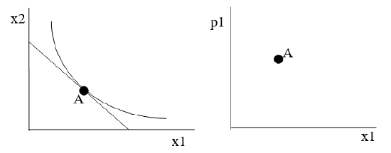 Figure 4.21: The initial solution.
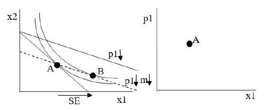 Figure 4.22: A
 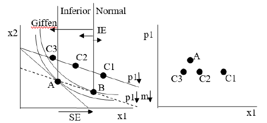 Figure 4.23: Understanding Giffen behavior.
 button and run Solver to make sure you are at the optimal initial solution of 44,11. Increase m to 60 and run Solver. What happens?