We began the Theory of Consumer Behavior with the Standard Model where cash income (m) is given. The Endowment Model replaced given cash income with an initial endowment of two goods so the budget constraint became \(p_1x_1 + p_2x_2 = p_1\omega _1 + p_2\omega _2\). We then focused on choices with badsrisky assets and accidents.
The application in this section is another example using a bad. As always, our eventual goal is comparative statics and elasticity. In this case, we will derive a supply curve for labor and concentrate on the wage elasticity of labor supply.
An innovation in this section is that the accompanying Excel workbook is less finished than usual. This enables you to practice implementing the model in Excel.
Setting Up the Problem
Instead of a mere consumer, the agent in this application is a consumer and worker.
Although an initial amount of non-labor income is assumed, total income can be increased by working. More hours at work means more income and greater consumption of goods and services. Consumption is good, but work is bad. Therein lies the problem.
Our consumer/worker can buy a single good, G, representing all consumer goods, at price p. Utility increases as she consumes more G.
The 24 hours in a day are divided into two types: work and leisure. The number of hours spent working in one day, H, is chosen by the agent. Earned income is simply \(wH\),where w is the wage rate in $/hr. Although work generates income, our agent does not like to work. H is a bad in the utility function.
With this background, we are ready to organize the information into the three areas that comprise an optimization problem:
Goal: maximize utility, which is a function of goods consumed, G, and work, H, where H is a bad.
Endogenous variables: G, the amount of goods consumed, and H, the number of hours worked.
Exogenous variables: p, the price of the composite good; w, the wage rate; m, unearned, non-labor income; and parameters in the utility function.
The solution to this constrained optimization problem is depicted on a graph with a budget constraint and set of indifference curves. We consider each of these elements separately and then combine them.
Budget Constraint
The budget constraint is \(m + wH \ge pG\). This equation says that total income is composed of unearned income (m) and earned income (\(wH\)). The inequality means that the consumer/worker cannot spend more on goods and services (\(pG\)) than the total income available.
Because no time elapses in this optimization problem, there is no reason for the agent to save (i.e., spend less than available) and we can make the constraint a strict equality, \(m + wH = pG\). This allows us to use the Lagrangean method to solve the problem analytically.
In terms of a graph, it is easy to see that we can write the constraint as the equation of a line (with G on the y axis and H on the x axis) by dividing by p: \[m + wH = pG\] \[G = \frac{m}{p}+\frac{wH}{p}\] Suppose w = $10/hr, m = $40, and p = $1/unit. What would the constraint look like?
STEP Open the Excel workbook LaborSupply.xls and read the Intro sheet, then go to the YourConstraint sheet.
Your task is to fill in the G column and create a chart of the constraint. There are three steps.
STEP Click on B12 and enter a formula equal to the equation for G. The cells w, p, and m are not named so you should use absolute references ($ in front of column letters and row numbers) to enable easy filling down of the formula.
When finished, the formula in B12 should look like this: = $B$4/$B$3 + ($B$2/$B$3)*A12.
STEP The next step is to fill down the formula.
STEP Finally, create a chart with H and G as the source data. Be sure to label the axes of your chart.
The chart is based on hour intervals of work, but fractions of hours are possible. Thus, your chart should be a scatter chart with points connected by lines.
STEP Click the button to see a finished version of the budget constraint.
The agent is free to choose any point on the constraint. The y intercept, 40 (equal to \(\frac{m}{p}\)), yields a small value of consumption, but the agent does not have to work. Movement up the line yields more G, but requires more H.
Points to the northwest of the line are unattainable. For example, the consumer/worker cannot afford the 10,200 combination. Working 10 hours adds $100 to the $40 non-labor income. This is not enough to buy $200 worth of goods.
What shock would enable our consumer/worker to buy the 10,200 combination?
There are three possibilities, one for each exogenous variable in the constraint.
STEP From the Constraint sheet (click the button from the YourConstraint sheet if needed), change the wage to 16 in B2.
The constraint rotates up, counterclockwise, with a steeper slope and the same intercept, and the combination 10,200 is now feasible, which is easily confirmed by looking at the chart and row 22.
Changes in wages, ceteris paribus, rotate the constraint around the unearned income intercept.
STEP Return the wage to 10 in B2 (the constraint returns to its initial position when you hit the Enter key) and set p (in B3) to 0.7.
Instead of raising the wage, we have made the composite good cheaper. As with a wage increase, this is welcome news since there are more consumption possibilities.
The constraint appears to simply rotate up again, but look more carefully at the chart and underlying data. The slope is steeper, but the intercept has also changed. The $40 of unearned income now buys a little more than 57 units of G. As before, it is easy to see that the combination 10,200 is now feasible.
Changes in price (p), ceteris paribus, rotate and shift the constraint.
STEP Return the price to 1 in B3 (the constraint returns to its initial position when you hit the Enter key) and set m (in B4) to 100.
This time, the constraint shifts vertically up. With $100 of unearned and $100 of earned income (from working 10 hours), the combination 10,200 is now feasible.
Changes in unearned income (m), ceteris paribus, shift the constraint.
Changes in w, p, and m affect the constraint. The initially unattainable combination of 10,200 can be made feasible by appropriately changing any of one of these three exogenous variables.
Preferences
In previous applications with bads, we used a Cobb-Douglas utility function and subtracted the bad from a constant. The same approach is adopted here.
Because the time period under consideration is a day, which has 24 hours, preferences can be represented by \(U(H, G) = (24 - H)^cG^d\).
With \(H = 0\), the agent gets the maximum value from the first term of the utility function, but remember that earned income will then be low and, therefore, G will be small.
Like the budget constraint, we need a visual representation of the utility function.
STEP Proceed to the YourIndiffCurve sheet to implement the utility function in Excel.
The sheet is unfinished. You need to fill in column B and draw a graph of the indifference curve. The indifference curve is initially based on \(c = d = 1\) and a level of utility of 1960.
To fill in column B, you need to solve for the value of G that yields a utility level of 1960, given H. In other words, rewrite the utility function in terms of G, like this:
STEP Use the expression above to enter a formula in B12 that computes the value of G necessary to produce a utility of 1960 when H = 2.
Your formula should look like this: = ($B$5/((24 - A12)(̂$B$3)))(̂1/$B$4). It evaluates to a value of \(G = 89.09\). This result makes sense because when H = 2, then \(24 - 2 = 22\) and 22 x 89.09 (since \(c=d=1\)) equals a utility value of 1960.
Notice again the use of absolute references.
STEP Fill down the formula and draw a chart with H and G as the source data. Label the axes.
Your chart is a graph of a single indifference curve. In fact, the entire quadrant is full of these upward sloping indifference curves and utility increases as you move in a northwesterly direction (taking less of the bad, H, and more of the good, G). This is the usual indifference map when we have a bad on the x axis.
Click the button to check your work or if you need help.
Finally, remember that changes in the exponents make the indifference curves flatter or steeper. A Q&A question explores this point.
Finding the Initial Optimal Solution
Having modeled the constraint and preferences, we are ready to find the initial solution.
The numerical approach is covered here; the analytical method is an exercise question.
STEP Proceed to the YourOptimalChoice sheet.
It is blank! You need to implement the problem in this sheet and run Solver to find the initial solution.
Organize the problem into the usual components: goal (maximize utility), endogenous variables (H and G), exogenous variables (\(w, p, m, c\), and d), and a cell for the constraint.
The utility function is \(U(H, G) = (24 - H)^cG^d\). The wage rate is $10/hr, the price of G is $1/unit, unearned income is $40, and \(c = d = 1\).
Click the button once you are finished or if you get stuck and need help.
Figure 6.8 shows the canonical graph of the initial optimal solution for the consumer/worker’s constrained utility maximization problem.
Figure 6.8: The initial solution.
Source: LaborSupply.xls!OptimalChoice
This consumer/worker maximizes utility by working 10 hours, thereby earning $100 and then buying 140 units of G. There is no better solution. Traveling up or down the budget constraint is guaranteed to lower utility because the indifference curve is just touching the constraint at 10,140. The mathematical way of saying this is that the MRS = \(\frac{w}{p}\) at 10,140.
Comparative Statics: Deriving Labor Supply
How does \(H \mbox{*}\) respond as the wage rate changes, ceteris paribus? This comparative statics question yields the labor supply curve.
We concentrate on the numerical approach and leave the analytical method for an exercise question.
STEP Proceed to the OptimalChoice sheet (in the YourOptimalChoice sheet, click the button if needed). Use the Comparative Statics Wizard to pick a few points off of the labor supply curve. Make the size of the change in the wage rate 10 and apply the default five shocks.
Use the CSWiz data to compute the wage elasticity of hours worked from \(w=\$10\) to $20/hr. Create a graph the supply and inverse supply of labor curves.
STEP Proceed to the CS1 sheet and scroll down (if needed) to check your work.
Notice the labor supply and inverse labor supply curves (scroll down if needed). The shape of the curve is intriguing. As wage rises, optimal H seems to level offit continues to increase, but ever more slowly.
Notice also that the computed wage elasticity of labor supply from w = 10 to 20 in E14 is quite small at 0.1. This means that hours worked is unresponsive to changes in wages.
Labor supply has been extensively studied and extremely small elasticities with respect to wage are commonly found (see McClelland and Mok (2012) for a review of the literature). Income and substitution effects explain this result.
STEP Return to the OptimalChoice sheet and click the button, then change the wage rate (in B16) from 10 to 20.
The budget constraint rotates up (counterclockwise) in the charta welcome change in consumption possibilities. The initial optimal solution, 10,140, is no longer optimal. The consumer/worker needs to re-optimize.
STEP Run Solver (with w = 20).
The new optimal solution is at H = 11. A 100% increase in the wage (from 10 to 20) has produced a total effect of a 1 hour, or 10%, increase in hours worked.
We can decompose this total effect into income and substitution effects by shifting down the budget line to cancel out the increased purchasing power of the wage increase. In other words, we need to draw in an imaginary, dashed line that goes through the initial solution, with a steeper slope caused by the higher wage.
We can use a modified version of the Income Adjuster Equation to determine the amount of income we need to take away. Recall that we determine how much income to change via \(\Delta m = x_1\Delta p_1\). In the labor supply model, \(x_1\) is obviously H, and the price is now the wage, but we also need a sign change. An increase in the wage increases consumption possibilities in the labor supply model so we need a minus sign to show that wage increases must be offset by income decreases. Below is our modified Income Adjuster Equation with values substituted in: \[\Delta m = (\Delta H \mbox{*})(-\Delta w)\] \[\Delta m=(10)(-10)=-100\] This says that we must lower unearned income by $100 to cancel out the increased purchasing power from the $10/hr wage increase.
STEP Confirm that w = 20 (in B16) and change m to \(-60\) (in B17).
Notice that the budget line goes through the initial combination, 10,140. The line is not dashed, but it should be. Remember that this budget line does not actually exist. No one is going to take $100 from the agent. We are doing this to decompose the total effect of the wage increase into the income and substitution effects.
STEP Run Solver with w = 20 and m = \(-60\).
\(H \mbox{*} = 13.5\) hours of work and Figure 6.9 shows the three effects.
Figure 6.9: Total, income, and substitution effects.
Source: LaborSupply.xls!OptimalChoice
The substitution effect is \(+3.5\), the movement from H = 10 (the initial optimal solution) to 13.5 (the optimal solution with the higher wage, but lower m). It is the horizontal movement from point A to B.
The income effect is \(-2.5\), the movement from H = 13.5 (point B) to H = 11 (point C). The negative sign is important. It says that when income rises, the agent buys less of the bad.
The total effect is, of course, the observed movement from point A to point C, a 1-hour increase in hours worked. This is what would actually be observed as the wage rose from $10/hr to $20/hr.
Figure 6.9 makes clear why the response of hours worked to a wage increase is inelasticthe income and substitution effects are working against each other. The fact that the relative price of goods for an hour of work is cheaper drives the agent to work and consume more (this is the substitution effect, from A to B). But the increase in purchasing power encourages the agent to work less (from B to C, the income effect). The total effect on hours worked is small when the two effects are added together.
In fact, the income and substitution effects can explain an even more curious phenomenon that has been observed in the real worldhours worked actually falling as wage rises. Figure 6.10 shows the underlying graph and derived labor supply curve for an unknown utility function. Unlike the labor supply derived from the Cobb-Douglas utility function, which was always positively sloped, the labor supply curve in Figure 6.10 is said to be backward bending. At low wages, increases in wage lead to more hours worked (such as from point 1 to 2), but the supply curve becomes negatively sloped when wages rise from point 2 to 3.
Figure 6.10: A backward bending supply curve.
We have already seen that the small wage elasticity from point 1 to 2 is caused by the income effect’s working against the substitution effect. The same explanation underlies the negative response in hours worked as wages rise from point 2 to 3. In this case, not only does the income effect oppose the substitution effect, it actually swamps it.
Figure 6.11 shows what happens when we are on the backward bending portion of the labor supply curve. The substitution effect always induces more hours worked as wages rise. This is the movement from A to B. The income effect, however, counters some of this increase in hours worked. We can afford to work less (from B to C) because the wage is higher. When we are on the backward bending portion of the labor supply curve, the income effect actually overcomes the substitution effect so that the total effect (A to C) is a reduction in hours worked as the wage rises. In Figure 6.11, any point C to the left of A yields a point on the backward bending portion of the labor supply curve.
Income and substitution effects when \(H \mbox{*}\) falls as w rises.
Wage rises and I work less sounds just about as weird as price rises and I buy more. Is this Giffen behavior?
No because the wage change is not an own price effect. Figure 6.12 shows \(p_1\) and \(p_2\) changes in the Standard Model where two goods are purchased given fixed income. On the left, the change in \(p_1\) produces an own effect on \(x_1\) and a cross effect on \(x_2\).If \(x_1\) rises as \(p_1\) rises, then \(x_1\) is Giffen. If \(x_2\) rises as \(p_1\) rises (notice the cross effect), however, that does not make \(x_2\) a Giffen good. We use the cross effect to say that the goods are substitutes (instead of complements). To determine whether \(x_2\) is Giffen, we have to use the graph on the right of Figure 6.12. If \(x_2\) rises as \(p_2\) rises (notice the own effect), then \(x_2\) is Giffen. In other words, we need an own price change to determine Giffenness.
Figure 6.12: Understanding own and cross effects.
Figure 6.12 makes clear that a change in the wage in the labor supply optimization problem is like a change in the price of \(x_2\) in the Standard Model. The wage change is like the graph on the right, with an upward sloping budget constraint. The rotation is around a fixed valuethe x intercept in the Standard Model and unearned income in the labor supply model. Thus, the change in wage is an own price effect for G (on the y axis) and a cross price effect for H (on the x axis).
Because a change in the wage exerts a cross effect on hours worked, we cannot say anything about Giffenness for hours worked. We could, however, say that G was Giffen if it fell when wage rose. That would really be weird. Look at the figures of income and substitution effects in this chapter and you will never find a final point C that lies below an initial point A. In fact, leisure (work’s counterpart) is usually treated as a normal good: higher income leads to more leisure (and less work).
Deriving the Labor Supply Curve
Labor Economics is a major field within Economics. As a course, it is usually offered as an upper-level elective, with Intermediate Microeconomics as a prerequisite. Labor supply and demand are fundamental concepts. The former is based on a model in which work is a bad (the opposite of leisure, which is a good) and a consumer/worker maximizes satisfaction subject to a budget constraint.
By changing the wage, ceteris paribus, we can derive a labor supply curve. Economists are well aware that labor supply is often quite insensitive to changes in wages. This is explained by the opposing substitution and income effects. The backward bending portion of the labor supply curve is observed when the income effect swamps the substitution effect. This is not Giffen behavior, however, because we are dealing with a cross (not own) price effect.
Exercises
Show all of your work.
Do your results for \(H \mbox{*}\) and \(G \mbox{*}\) agree with the numerical approach in the text? Is this surprising?
Using the Comparative Statics Wizard, the wage elasticity of labor supply from $10/hr to $20/hr is 0.1. Use your reduced form solution for \(H \mbox{*}\) to find the wage elasticity of labor supply at w = $10/hr. Show your work.
Does your point wage elasticity from the previous question equal 0.1 (the wage elasticity based on a $10 wage increase)? Why or why not?
Whether the labor supply curve is upward sloping or backward bending has nothing to do with the Giffenness of work. If labor supply is positively sloped, G and H are substitutes or complements, but which one? Draw a graph that helps you explain your answer.
References
The epigraph comes from page 355 of Max Weber’s classic, General Economic History, originally published in German in 1923 and translated to English by Frank H. Knight in 1927. If you are unfamiliar with Weber (pronounced vay-ber), he was interested in the way capitalism changed people’s minds and values, especially how it made people more rational and calculating.
With respect to labor supply, the consumer/worker’s goals and attitudes are a critical issue. In this chapter, labor supply was derived as the solution to an optimization problem. The agent, however, might not be an optimizer, but a target earner, working only enough hours to make a certain amount of money. If wages double, hours worked are cut in half. If everyone was a target earner, the typical way to attract more workerspay morewould not work.
Consider this abstract from Henry Farber’s 2003 NBER working paper, “Is Tomorrow Another Day? The Labor Supply of New York Cab Drivers”:
I model the labor supply of taxi drivers as the result of optimization based on an inter-temporal utility function. Since income effects in response to temporary fluctuations in daily earnings opportunities are likely to be small, cumulative hours will be much more important than cumulative income in the decision to stop work on a given day. However, if these income effects are large due to very high discount and interest rates, then labor supply functions could be backward bending, and, in the extreme case where the wage elasticity of daily labor supply is minus one, drivers could be target earners. Indeed, Camerer, Babcock, Lowenstein, and Thaler (1997) and Chou (2000) find that the daily wage elasticity of labor supply of New York City cab drivers is substantially negative and conclude that it is likely that cab drivers are target earners. I conclude from my empirical analysis, based on new data, of the stopping behavior of New York City cab drivers that, when accounting for earnings opportunities in a reduced form with measures of clock hours, day of the week, weather, and geographic location, cumulative hours worked on the shift is a primary determinant of the likelihood of stopping work while cumulative income earned on the shift is weakly related, at best, to the likelihood of stopping work. This is consistent with there being inter-temporal substitution and inconsistent with the hypothesis that taxi drivers are target earners.
Google Scholar has tens of thousands of papers on Uber and how drivers decide how many hours to work.
Robert McClelland and Shannon Mok’s 2012 working paper that summarizes the wage elasticity literature, "A Review of Recent Research on Labor Supply Elasticities," is freely available from the Congressional Budget Office at www.cbo.gov/publication/43675. A remarkable finding is that men’s much larger substitution effect than women’s has all but disappeared so that men and women today respond similarly to wage shocks.


 button to see a finished version of the budget constraint.
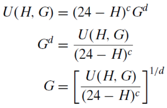
 button to check your work or if you need help.
 button once you are finished or if you get stuck and need help.
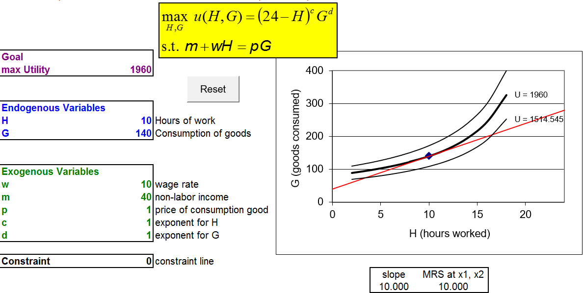
 button if needed). Use the Comparative Statics Wizard to pick a few points off of the labor supply curve. Make the size of the change in the wage rate 10 and apply the default five shocks.
 button, then change the wage rate (in B16) from 10 to 20.
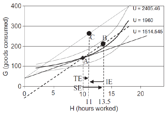
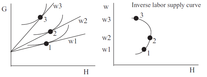 Figure 6.10: A backward bending supply curve.
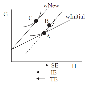
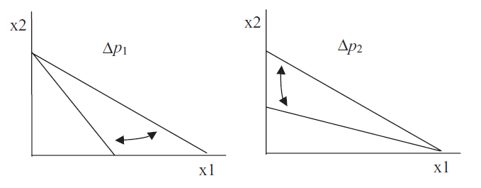 Figure 6.12: Understanding own and cross effects.