The Theory of Consumer Behavior is based on the idea that buyers choose how much to buy based on preferences, income, and given prices. We know, however, that buyers do not face a single pricethere is a distribution of prices and sellers change their prices frequently.
You would think consumers would be unable to choose in such an environment. After all, how can they know the budget constraint without prices? The answer is that they search or, in other words, they go shopping, and then use the lowest prices found to solve their constrained utility maximization problem.
Search Theory is an application of the economic approach to the problem of how long to shop in a world of many prices. Search is a productive activity because it enables one to find lower prices, but it is costly. One can search too little, ending up paying a high price, or search too muchspending hours to find a price that is a few pennies lower does not make much sense.
This chapter introduces the consumer’s search optimization problem and is based on the idea that consumers decide in advance how many price quotes to obtain, according to an optimal search rule. This type of search procedure is known as a fixed sample search.
Describing the Search Optimization Problem
We assume that consumers do not know the prices charged by each firm. We simplify the problem by assuming that the product in different stores is identical (i.e., homogeneous) so the consumer just wants to buy at the lowest price. Unfortunately, finding that lowest price is costly so the buyer has to decide how long to search.
STEP Open the FixedSampleSearch.xls workbook and read the Intro sheet, then proceed to the Setup sheet.
The first task is to create the distribution of prices faced by the consumer. We assume that prices remain fixed during the search process.
STEP Click the button.
You will be asked a series of questions that will establish the prices charged by all of the sellers. This is the population. The idea is that consumer will sample (draw) from the population. This is shopping.
STEP Hit OK when asked the number of stores selling the product to accept the default number of 1000 (no comma separator when entering numbers in Excel). Choose Uniform for the distribution and then press OK to accept 5 when prompted for the number of stores. Accept the default values of 0 and 1 for the minimum and maximum prices.
After you hit Enter, you will see a column of red numbers in column A that represent the prices charged by each of the 1,000 stores selling the product. The consumer knows that stores charge different prices, but cannot immediately see each individual store price. They cannot see the lowest and highest price stores in cells B2 and B3.
STEP Scroll down to see the prices charged at each store and confirm that the minimum price store, displayed in cell F2, is correct.
It is difficult to see by simply scrolling down and looking at the prices, but the uniform distribution you used means that prices are scattered equally from zero to one. The normal distribution, on the other hand, would concentrate prices near the average, with fewer low and high prices (like a bell-shaped curve). The log-normal is the most realistic of the threeprices have a long right-hand tail (with a few stores charging very high prices). The primary advantage of the uniform distribution is that it is the easiest to work with analytically.
Figure 7.1 shows a histogram of 1,000 prices from U[0,1]. This notation means that we include the endpoints so we have a uniform distribution with a zero minimum and a maximum of one (giving an average of 0.5 and an SD of 0.2887).
Figure 7.1: An example uniform distribution of prices.
The prices are not exactly evenly distributed on the interval from zero to one. They are drawn from a uniform distribution on the interval 0 to 1, but each realization of 1,000 prices deviates from a purely rectangular distribution due to randomness in sampling from the uniform distribution. The more stores you include in the population, the closer Figure 7.1 will get to a smooth, rectangular distribution. You can see a histogram of your population prices by scrolling over to column AA of the Setup sheet.
Consumers know the distribution of prices, but they do not know which firm is charging which price, so they cannot immediately go to the firm that has the lowest price. Instead, the fixed sample search model says that the consumer chooses a number of prices to sample (which you set as 5) and then chooses the lowest of the observed prices.
STEP Click the button. A price will appear in the sample column, and a pop-up box tells you where that price came from. Hit OK each time the display comes up. You will hit OK five times because you chose to sample from five stores.
The consumer chooses among the 1,000 stores randomly and ends up with five observed prices. Column L reports the sample average price, the SD of the sampled prices, and the minimum price in the sample (in cell L7). The consumer will purchase the product at the minimum price observed in the sample.
Why doesn’t the consumer visit every store and then pick the lowest price? Because it is costly to obtain price information, as shown in cell L11. Each shopping trip (to collect a price) costs 4 cents. To sample all 1,000 stores would cost the consumer an exorbitant $40. On average, the consumer would pay $0.54 (the average of the price distribution plus the cost of obtaining one price) by buying the product at the very first store visited. Clearly, it is better to buy immediately, n = 1, than to sample every store, n = 1,000, but what about other fixed sample sizes? How much will the consumer pay, on average, when sampling five stores?
STEP Hit the button repeatedly to draw more samples of size five. Keep your eye on the total price paid in cell L22.
Every time you get a new sample, you get a new total price (composed of the minimum price in sample plus 20 cents). There is no doubt about itthe total price the consumer ends up paying is a random variable. This makes this problem difficult because we need to figure out what the consumer can expect to pay usually or typically. We want to know the average total price. The next section shows how.
Monte Carlo Simulation
The plan is to alter the spreadsheet so a new sample can be drawn simply by recalculating the sheet, which is done by hitting the F9 key. We can then install the Monte Carlo simulation add-in and use it to repeatedly draw new samples, tracking the lowest price in each sample.
STEP Select cell range J2:J6. You should have five cells highlighted. In the formula bar, enter the following formula:
=DRAWSAMPLEARRAY()
and then press Ctrl + Shift + Enter (hold down and continuing holding down the Ctrl key, then hold down and continue holding down the Shift key, and then hit the Enter key). Your sample of five prices will appear in the sample column.
After you select the cells, do not simply hit the Enter key. This will put the formula only in the first cell. You want the formula in all five cells that you selected. You have to press Ctrl + Shift + Enter simultaneously.
You have used an array function (built into the workbook) that spans the five cells you selected. You cannot individually edit the cells. If you mistakenly try to do so and get stuck, hit the esc (escape) key to return to the spreadsheet.
When using this array function, it may display #VALUE. Simply hit the F9 key when this happens to refresh the function. If that does not work, recreate the population.
When using the DRAWSAMPLEARRAY() function, you must be sure to set the number of draws in cell C15 to correspond to the number of cells selected and used by the function. If there is a discrepancy, a warning will be displayed.
STEP Hit F9 a few times and keep your eye on cells L7, the minimum price, and L22, the total price paid.
These cells update each time you hit F9. A new sample of five prices is drawn and the minimum price and total price paid are recalculated for the new sample.
The DRAWSAMPLEARRAY() function enables Excel to display the minimum (best) price random variable, but we need to figure out the average minimum price when five price quotes are obtained. This can be done by repeatedly resampling and tracking each outcome – this is called Monte Carlo simulation.
STEP Install the Monte Carlo simulation Excel add-in, MCSim.xla, available freely from www3.wabash.edu/econometrics and the MicroExcel archive (in the same folder as the Excel workbook for this section). Full documentation is available at this web site. This powerful add-in enables sophisticated simulations with the click of a button.
Remember that installing an add-in requires use of the Add-ins Manager. Do not simply open the MCSim.xla file.
Once installed, you can use the add-in to determine the average minimum price and total price paid for the product when five prices are sampled.
STEP Run the Monte Carlo simulation add-in on cells L7 and L22 with 10,000 repetitions.
Your MCSim add-in dialog box should look like Figure 7.2. Click the button to run the simulation.
Figure 7.2: Configuring the MCSim dialog box.
Your simulation results will look something like Figure 7.3, but your results will be slightly different. The average of the minimum price distribution should be near 0.17 (1/6). Thus, the consumer will usually pay around $0.37 (adding the 20 cents in search cost) for the product. The total price paid is a shifted version of the best price.
Figure 7.3: Monte Carlo simulation results with n = 5.
Source: FixedSampleSearch.xls!MCSim
So now we know that the consumer can expect to pay about $0.37 when searching five stores. This is better than buying at the first store visited, which was $0.54. Compared to the buying at the first store, the expected marginal gain of shopping at five stores, in terms of a lower expected minimum price, is \(\$0.50 - \$0.17 = \$0.33\). The additional cost of searching for five prices instead of one is $0.16. The additional benefit is greater than the additional cost is another way to know that five stores is better than one store.
But we want to know more than just that searching five stores is better than buying at the first store; we want to find the best sample sizethe one that gives the lowest total price paid.
STEP Hit the button. Change the number of draws in cell C15 to 10. Select cell range J2:J11 and then type in the formula bar: =DRAWSAMPLEARRAY(). Then press the Ctrl + Shift + Enter combination to input the array formula. Your sample of 10 prices will appear in column J.
Hit F9 a few times and watch what happens to cell L7, the minimum price. It bounces, but with 10 prices instead of five, it bounces around a different, lower mean.
STEP To find the typical price the consumer can expect to pay, run a Monte Carlo simulation of the minimum and total price when 10 stores are visited.
Figure 7.4 shows the exact average best price and average total price as a function of the sample size for the U[0,1] price distribution. Your simulation results for the best price for n = 10 should be close to $0.0909.
Figure 7.4: Optimal Search with a Uniform Distribution on the interval [0,1].
Source: FixedSampleSearch.xls!Summary
The typical $0.0909 best price when 10 prices are obtained is lower than when we shopped at five stores, but notice that it isn’t worth it. The cost of obtaining 10 prices ($0.40) is so high that the total price paid is higher than getting just five prices. In fact, getting four prices is the optimal sample size.
Analytical Methods
The optimal search optimization problem can be solved via analytical methods. For the uniform price distribution on the interval from zero to one, the average minimum price in the consumers’ hands after visiting n firms is \[AverageP_{min}=\frac{1}{n+1}\] The equation for the average minimum price shows that it is decreasing as n rises and it does so at a decreasing rate. In other words, there are diminishing returns to searching for low prices.
The consumer’s optimization problem is to minimize the expected total cost of acquiring the product, where \(P(n)\) represents the expected minimum price that we know is a function how many prices are collected: \[\min\limits_{n}TC=P(n)q +cn\] We also know that for U[0,1], \(P(n)=\frac{1}{n+1}\) so we have: \[\min\limits_{n}TC=\frac{1}{n+1}q +cn\] To find optimal n, take the derivative with respect to n and set it equal to zero: \[\frac{dTC}{dn}=-\frac{1}{(n+1)^2}q +c =0\] \[\frac{1}{(n+1)^2}q = c\] This equimarginal condition says that the optimal sample size is found where marginal savings from additional search equals marginal cost. As long as the savings from searching an additional store exceeds the cost of collecting one more price, the consumer will continue to search. The marginal savings is just the drop in the expected price, times the number of units that the consumer wants to purchase.
From the equimarginal condition, we can solve for optimal n to get a reduced form solution. \[\frac{1}{(n+1)^2}q = c \rightarrow q=c(n+1)^2 \rightarrow \sqrt{\frac{q}{c}}=n+1 \rightarrow \sqrt{\frac{q}{c}}-1=n \mbox{*}\] With q = 1 and c = $0.04, we have the same solution we found earlier: \[n \mbox{*}=\sqrt{\frac{q}{c}}-1=\sqrt{\frac{1}{0.04}}-1=4\]
Comparative Statics
The reduced form expression makes comparative statics analysis straightforward. It is obvious that higher c, search cost, leads to lower optimal sample size, as shown in Figure 7.5.
Figure 7.5: Optimal search with changing search cost for q = 1.
Search cost is not the same for each consumer. Time is an important element of search cost. Those with more valuable time and, therefore, higher search cost will optimize by obtaining fewer price quotes.
The availability of information is another component of search cost. Informational advertising is how firms let consumers know where they are and what prices are being charged. We can model this type of advertising as a decrease in search coststoday, all the consumer has to do is go online to see what prices are being offered. Search costs are still positive (consumers do not know, for example, whether all firms advertise or just some), but lower than without advertising. Consumers obtain the product for a lower total price when advertising lowers search costs.
If we allow for multiple purchases, that is, a value of q\(> 1\), then the returns to search increase and, other things equal, the optimal number of searches increases. The effect of increasing q on the relationship between the cost of search and the optimal number of searches is shown in Figure 7.6.
Figure 7.6: Optimal search with changing n and q.
For example, the driver of an 18-wheel truck that carries two 200-gallon diesel tanks is going to search more than someone looking to fill her car with gas. But this example leads to the next chapter, where we introduce a different search model.
Results of Fixed Sample Search
Incomplete price information leads to an entirely new optimization problem. Because consumers will not search every store, since that is too expensive, we see price dispersion. This is a major result of search theory and it deserves further explanation.
You would think that competition would tend to make prices of the same product equal. This is known as the Law of One Price. But this only applies to a world where consumers can costlessly gather prices.
In other words, the Law of One Price will fail to hold whenever it is costly to collect price data. This is true in the real world, where some consumers will end up paying higher prices than others because the minimum price in their particular information set is different than the minimum price in another consumer’s set.
Because lower search costs induce more search, a reduction in search costs would have the effect of reducing (but not eliminating) price dispersion. Because optimizing consumers will choose not to canvass every store for prices as long as search is costly, price dispersion will exist. This is the key result of the fixed sample search model.
Economists have been interested in search theory for decades. The internet promised a big decrease in search cost and it may well have delivered that, but more recently, technology has really upended search theory. Today, your online search behavior is monitored and your clicks influence the prices you see.
The next level search models do not treat the population of prices as given and do not allow the consumer to randomly sample without changing the price distribution. Consumers still have an optimization problem to solve, but so do firms.
Exercises
Suppose the price distribution of 1,000 firms is uniform, with an average price of $50 and an SD of $28.87. Search cost, c, is $1 per price.
On what interval (from the minimum to the maximum) are prices equally likely to fall?
Implement this problem in the Setup sheet and run a Monte Carlo simulation with a sample size of 20. Take a picture of your results (like Figure 7.3) and paste it in a Word document. What is good about obtaining 20 prices? What is bad?
Use the equation for the average minimum price as a function of n for this distribution, \(AverageP_{min}=\frac{100}{n+1}\), to find the optimal sample size. Show your work.
Find the c elasticity of n at \(q = c = 1\). Show your work.
References
The epigraph is from page 214 of George J. Stigler, “The Economics of Information,” The Journal of Political Economy, Vol. 69, No. 3 (June, 1961), pp. 213–225, www.jstor.org/stable/1829263. This paper is recognized as the beginning of the economics of search.
Stigler was trying to explain price dispersion, but search theory has expanded far beyond this and is especially important in Labor economics. A consumer shopping for a low price product is the same as a worker looking for a high wage job or a firm seeking a high quality employee. See Richard Rogerson, Robert Shimer, and Randall Wright, “Search-Theoretic Models of the Labor Market: A Survey,” Journal of Economic Literature, Vol. 43, No. 4 (December, 2005), pp. 959–988, www.jstor.org/stable/4129380.


 button.
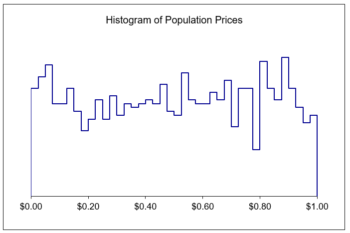 Figure 7.1: An example uniform distribution of prices.
 button. A price will appear in the sample column, and a pop-up box tells you where that price came from. Hit OK each time the display comes up. You will hit OK five times because you chose to sample from five stores.
 button repeatedly to draw more samples of size five. Keep your eye on the total price paid in cell L22.
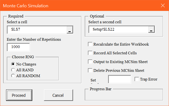 Figure 7.2: Configuring the MCSim dialog box.
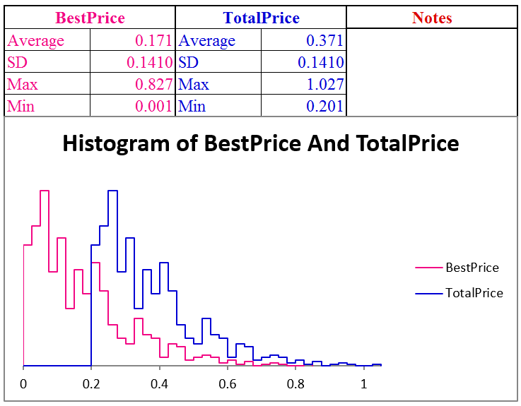
 button. Change the number of draws in cell C15 to 10. Select cell range J2:J11 and then type in the formula bar: =DRAWSAMPLEARRAY(). Then press the Ctrl + Shift + Enter combination to input the array formula. Your sample of 10 prices will appear in column J.
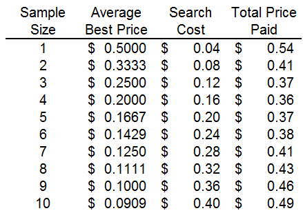
 Figure 7.5: Optimal search with changing search cost for q = 1.
 Figure 7.6: Optimal search with changing n and q.