7.2: Sequential Search
- Last updated
- Jul 17, 2023
- Save as PDF
- Page ID
- 58469
( \newcommand{\kernel}{\mathrm{null}\,}\)
We introduced Search Theory with a Fixed Sample Search Model. A consumer samples from the population of stores and gets a list of n prices for a product, then chooses the minimum price. The bigger n, the lower the minimum price in the list, but the price paid to obtain the price quotes increases as n rises. The consumer has to decide how many prices to obtain.
This section explores the properties of a different situation that is known as the Sequential Search Model. Unlike fixed sample search, where the consumer obtains a set of price quotes and then picks the lowest price, sequential search proceeds one at a time. The consumer samples from the population and gets a single price, then decides whether or not to accept it. If she rejects it, she cannot go back. As the epigraph shows, the sequential search model is easily applied to job offers, but it will be applied in this chapter to another common search problembuying gas.
Setting Up the Model
Imagine you are driving down the road and you need fuel. As you drive, there are gas stations (say N = 100) to the left and right (taking a left does not bother you too much) and you can easily read the price per gallon as you drive up to each station. If you drive past a station, turning around is out of the question (there is traffic and you have a weird phobia about U-turns).
There is a lowest price station and the stations can be ranked from 1 (lowest, best price) to 100 (highest, worst price). You do not know the prices coming up because the stations are randomly distributed on the road. The lowest price station might be 18th or 72nd or even the very first one. Figure 7.7 sums it all up.
 Figure 7.7: Deciding where to buy gas.
Suppose you focus on the following question: How do you maximize the chances of finding the cheapest station?
You might argue that you should drive by all of the stations, and then just pick the best one. This is a terrible idea because you cannot go back (remember, no U-turns). Once you pass a station, you cannot return to it. So, this strategy will only work if the cheapest station is the very last one. The chances of that are 1 in a 100.
A strategy for choosing a station goes like this: Pick some number K<N where you reject (drive by) stations 1 to K, then choose the first station that has a price lower than the lowest of the K stations that you rejected.
Perhaps K = 50 is the right answer? That is, drive by stations 1 to 50, then look at the next (51st) station and if it is better than the lowest of the 50 you drove by, pull in. If not, pass it up and consider the 52nd station. If it is cheaper than the previous 51 (or 1 to 50 since we know the 51st station isn’t cheaper than the cheapest of the first 50), get gas there.
Continue this process until you get gas somewhere, pulling into the last (100th) station if you get to it (it will have a sign that says, “Last chance gas station”).
This strategy will fail if the lowest price is in the group of the K stations you drove by, so you might want to choose K to be small. But if you choose K too small, you will get only a few prices and the first station with a price lower than the lowest of the K stations is unlikely to give you the lowest price.
So, K = 3 is probably not going to work well because you probably won’t get a super low price in a set of just three so you probably won’t end up choosing the lowest price. For example, say the first three stations are ranked 41, 27, and 90. Then as soon as you see a station better than 27, you will pull in there. That might be 1, but with 26 possibilities, that’s not likely.
On the other hand, a high value of K, say 98, suffers from the fact that the lowest price station is probably in that group and you’ve already rejected it! Yes, this problem is certainly tricky.
The Sequential Search Model can be used for much more than buying gasit has extremely wide applicability and, in math, it is known as optimal stopping. In hiring, it is called the secretary problem. A firm picks the first K applicants, interviews and rejects them, then picks the next applicant that is better than the best of the K applicants. It also applies to many other areas, including marriagesearch online for Kepler optimal stopping to see how the famous astronomer chose his spouse.
STEP Open the Excel workbook SequentialSearch.xls and read the Intro sheet, then proceed to the Setup sheet.
Column A has the 100 stations ranked from 1 to 100. The lowest priced station is 1, and the highest priced station is 100.
STEP Click the  button. It shuffles the stations, randomly distributing them along the road you are traveling in column D.
Cell B7 reports where the lowest priced station (#1) is located. Columns C and D report the location of each station. Column D changes every time you click the  button because the stations are shuffled.
Cell F2 sets the value of K. This is the choice variable in this problem. Our goal is to determine the value of K that maximizes the probability that we get the lowest priced station.
On opening, K = 10. We pass up stations 1 to 10, then take the next station that is better than the best of the 10 stations we rejected.
STEP Click the  button. This reshuffles the stations and draws a border in column D for the cell at the Kth station.
Cell F5 reports the best of the K stations (that were rejected). Cell F7 displays the station you ended up at.
STEP Scroll down to see why you ended up at that station and read the text on the sheet.
Cell F7 always displays the first station that is better (lower) than the best of the K stations in cell F5.
STEP Repeatedly click the  button. After every click, see how you did. Is 10 a good choice for K?
The definition of a good choice in this case is one that has a high probability of giving us the cheapest station. Our goal is to maximize the chances of getting the cheapest station. We could have a different objective, for example, minimize the average price paid, but this would be a different optimization problem. For the classic version of the optimal stopping problem, we count success only when we find the cheapest station.
STEP Change K to 60 (in F2) and repeatedly click the  button. Is 60 better than 10?
This is difficult to answer with the Setup sheet. You would have to repeatedly hit the  button and keep track of the percentage of the time that you got the cheapest station. That would require a lot of patience and time tediously clicking and recording the outcome. Fortunately, there is a better way.
Solving the Problem via Monte Carlo Simulation
The Setup sheet is a good way to understand the problem, but it is not helpful for figuring out the optimal value of K. We need a way to quickly, repeatedly sample and record the result. That is what the MCSim sheet does.
STEP Proceed to the MCSim sheet and look it over.
With N = 100 (we can change this parameter later), we set the value of K (in cell D7) and run a Monte Carlo simulation to get the approximate chances of getting the best station (reported in cell H7).
Unlike the MCSim add-in used in the previous section, this Monte Carlo simulation is hard wired into this workbook. Thus, it is extremely fast.
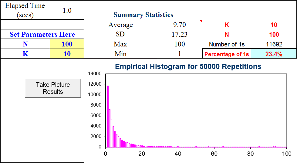
STEP With N = 100 and K = 10, click the  button. The default number of repetitions is 50,000, which seems high, but a computer can do hundreds of thousands of repetitions in a matter of seconds.
Figure 7.8 shows results. Choosing K = 10 gives us the best station about 23.4% of the time. Your results will be slightly different.

Figure 7.8: Monte Carlo simulation results.
Source: SequentialSearch.xls!MCSim
Notice that we are using Monte Carlo simulation to approximate the exact answer. Monte Carlo simulation cannot give us the exact answer. By increasing the number of repetitions, we improve the approximation, getting closer and closer, but we can never get the exact truth with simulation. The answer it gives depends on the actual outcomes in that particular run. The only way simulation would give the exact answer is if it was based on an infinite number of repetitions.
Can we do better than getting the best station about 23% of the time?
We can answer this question by exploring how the chances of getting the lowest price varies with K. By changing the value of K and running a Monte Carlo simulation, we can evaluate the performance of different values of K.
STEP Explore different values of K and fill in the table in cells J3:M10.
As soon as you do the first entry in the table, K = 20, you see that it beats K = 10.
STEP Use the data in the filled in table to create a chart of the chances of getting the lowest price station as a function of K. Use the button under the table to check your work.
What do you conclude from this analysis?
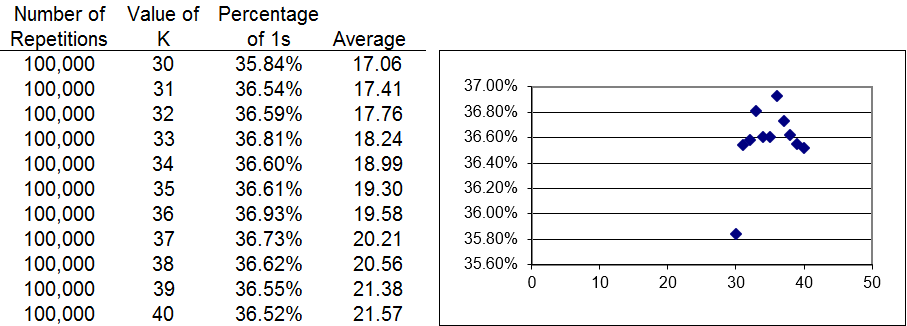
One problem with Monte Carlo simulation is the variability in the results. Each run gives different answers since each run is an approximation to the exact answer based on the outcomes realized. Thus, it seems pretty clear that the optimal value of K is between 30 and 40, but using simulation to find the exact answer is difficult.
Figure 7.9 displays results of series of Monte Carlo experiments. Notice that we doubled the number of repetitions to increase the resolution. The best value of K appears to be 36, but the noisiness in the simulation results makes it impossible to determine the answer.

Figure 7.9: Zooming in on the value of optimal K.
Source: SequentialSearch.xls!Answers
With Monte Carlo simulation, we can continue to increase the number of repetitions to improve the approximation.
STEP Proceed to the Answers sheet to see more simulation results.
The Answers sheet shows that even 1,000,000 repetitions are not enough to definitively give us the correct answer. Simulation is having a difficult time distinguishing between a stopping K value of 36 or 37.
An Exact Solution
This problem can be solved analytically. The solution is implemented in Excel. For the details, see the Ferguson citation at the end of this chapter.
STEP Proceed to the Analytical sheet to see the exact probability of getting the cheapest station for a given K-sized sample from N stations from 5 to 100.
For example, cell G10 displays 32.74%. This means you have a 32.74% probability of getting the cheapest station out of 10 stations if you drive by the first six stations and then choose the next station that has a price lower than the cheapest of the K stations you drove by.
For N = 10, is K = 6 the best solution?
No. The probability of choosing the cheapest station rises if you choose K = 5. The 3 and 4 choices are close, but clearly, optimal K = 3 (with a 39.87% likelihood of getting the cheapest station) is the best choice.
In the example we have been working on, we had N = 100. Monte Carlo simulations showed optimal K around 36 or 37, but we were having trouble locating the exact right answer.
STEP Scroll down to see the probabilities for N = 100. Click on cells AL100 and AM100 to see the exact values. The display has been rounded to two decimal (percentage) places, but the computation is precise to more decimal places.
K* = 37 just barely beats out K = 36. The fact that they almost give the exact same chances of getting the lowest price explains why we were having so much trouble zooming in on the right answer with Monte Carlo simulation.
It can be shown (see the Ferguson source in the References section) that optimal K is Ne, giving a probability of finding the cheapest station of 1e. For N = 100, Ne≈36.7879.
If K was a continuous endogenous variable, Ne would be the optimal solution. But it is not, so the exact, correct answer is to pass on the first 37 stations and then take the first one with a lower price than the lowest price of stations 1 to 37.
It is a mystery why the transcendental number e, the base of natural logarithms, plays a role in the solution.
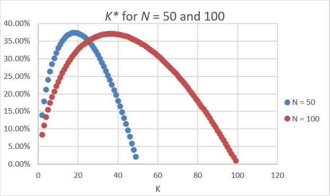
Figure 7.10 shows that as N rises, so does optimal K. What elasticity is under consideration here?

Figure 7.10: Exact probabilities of finding the cheapest station.
Source: SequentialSearch.xls!Analytical
The answer is the N elasticity of K. From N = 50 to 100 is a 100% increase. What happens to optimal K? It goes from 18 to 37, so a little more than a 100%. The elasticity is slightly over one. If you use the continuous version of K, then K exactly also doubles and the N elasticity of K is exactly one.
Sequential Search Lessons
Unlike the Fixed Sample Search Model (where you obtain a set of prices and choose the best one), the Sequential Search Model says that you draw sample observations one after the other. This could apply to a decision to choose a gas station. As you drive down the road, you decide whether to turn in and get gas at Station X or pass up that station and proceed to Station Y.
Faced with price dispersion, a driver deciding where to get gas can be modeled as solving a Sequential Search Model. Although there can be other objectives (such as getting lowest average price), the goal could be to maximize the chances of getting the lowest price. We found that as N rises, so does optimal K. The more stations, the more driving you should do before picking a station.
Like the Fixed Sample Search Model, the Sequential Search Model does not have any interaction between firms and consumers. Price dispersion is given and the model is used to analyze how consumers react in the given environment.
In the pre-internet and smartphone days, deciding where to get gas was quite the challenge. A driver passing signs with prices (like Figure 7.7) was a pretty accurate representation of the environment. There was no Google maps or apps displaying prices all around you. Notice, however, that the Law of One Price does not yet apply to gas prices.
Ferguson points out that our Sequential Search Model (which mathematicians call the secretary problem) is part of a class of finite-horizon problems. "There is a large literature on this problem, and one book, Problems of Best Selection (in Russian) by Berezovskiy and Gnedin (1984) devoted solely to it" (Ferguson, Chapter 2).
Fixed Sample and Sequential Search Models are merely the tip of the iceberg. There is a vast literature and many applications in the economics of search, economics of information, and economics of uncertainty.
Exercises
- Use the results in the Analytical sheet to compute the N elasticity of K* from N = 10 to 11. Show your work.
- Use the results in the Analytical sheet to draw a chart of K* as a function of N. Copy and paste your graph in a Word document.
- Run a Monte Carlo simulation that supports one of the N-K* combinations in the Analytical sheet. Take a picture of your simulation results and paste it in a Word document.
- Explain why the Monte Carlo simulation was unable to exactly replicate the percentage of times the lowest priced station was found.
References
The epigraph is from pages 115 and 116 of J. J. McCall, "Economics of Information and Job Search," The Quarterly Journal of Economics, Vol. 84, No. 1 (February, 1970), pp. 113–126, www.jstor.org/stable/1879403. This paper shows that sequential search (with recall) dominates fixed sample search. For more on this point, see Robert M. Feinberg and William R. Johnson, "The Superiority of Sequential Search: A Calculation," Southern Economic Journal, Vol. 43, No. 4 (April, 1977), pp. 1594–1598, www.jstor.org/stable/i243526.
Thomas Ferguson, Optimal Stopping and Applications is freely available online at www.math.ucla.edu/ tom/Stopping/Contents.html. Ferguson offers a technical, mathematical presentation of search theory.
C. J. McKenna, The Economics of Uncertainty (New York: Oxford University Press, 1986), is a concise, nontechnical introduction to imperfect information models.
John Allen Paulos, Beyond Numeracy (New York: Alfred A. Knopf, 1991), p. 64, discusses the optimal interview problem with an easy, intuitive style.


