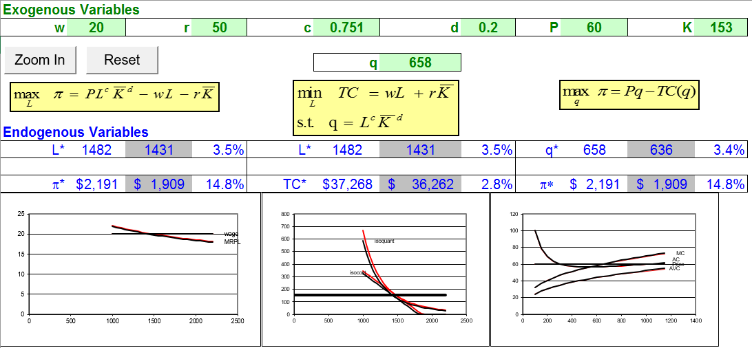
We have considered three separate optimization problems in our study of the perfectly competitive (PC) firm. Figures 14.1, 14.2, and 14.3 provide a snapshot of the initial solution and the key comparative statics analysis from each of the three optimization problems.
This chapter ties things together with the fundamental point that these three problems are tightly integrated and are actually different views of the same firm and same optimal solution. Change an exogenous variable and all three optimization problems are affected. The new optimal solutions and comparative statics results are consistenti.e., they tell you the same thing and are never contradictory.
Figure 14.1 shows the input side cost minimization problem. Quantity is exogenous in this problem and the firm looks for the input mix that minimizes the total cost of producing the given q.
Figure 14.1: Initial cost minimization and cost function.
The right panel in Figure 14.1 shows the cost function that comes from tracking minimum total cost as q varies, ceteris paribus.
Figure 14.2 shows output side profit maximization. The PC firm (since \(P=MR\) is a horizontal line) gets average and marginal cost curves from the cost function and finds the quantity that maximizes profit.
Figure 14.2: Initial profit maximization and the supply curve.
The right panel in Figure 14.2 shows where supply curves come from: shock P, ceteris paribus, and track optimal q.
Figure 14.3 returns to the input side, but this time the firm solves a profit maximization problem, choosing how much labor to hire.
Figure 14.3: Initial profit maximization and the demand for labor.
The right panel in 14.3 shows how changing w, ceteris paribus, produces the demand curve for labor.
These three optimization problems share a common methodology. In each case, we set up and solve the problem, then do comparative statics analysis. There are other shocks that can be explored, but the one shown here is the most important.
But there is one last crucial concept that is the focus of this chapter: these three problems do not exist in isolation, instead, they are woven together to comprise the Theory of the Firm. The relationships among the three exhibit a consistency that can be demonstrated with Excel.
Perfect Competition in the Long Run
STEP Open the Excel workbook Consistency.xls and read the Intro sheet; then proceed to the TheoryoftheFirmLongRun sheet. Use the button to fit the graphs on your screen so that all of them can be seen simultaneously.
The first and most important point is that all three optimization problems, in unison, comprise the Theory of the Firm. Perhaps because they see it in introductory economics, many students think of the output profit maximization graph as the firm. The display in Consistency.xls gives a strong visual presentation and constant reminder that the firm has three facets.
Gray-backgrounded cells are dead (click on one to see that it has a number, not a formula). They serve as benchmarks for comparisons when we do comparative statics.
The output and input profit maximization graphs do not have the usual U-shaped curves because the production function is Cobb-Douglas. This functional form cannot generate conventional U-shaped MC and AC curves (or upside down U-shaped MRP and ARP). There is no separate AVC curve because we are in the long run, so \(AC = AVC\).
STEP Compare the initial solutions for each of the three problems.
There are several ways in which they agree.
\(L \mbox{*}\) and \(K \mbox{*}\) are the same in the Input Profit Max (left) and Input Cost Min (middle) graphs.
If you use these amounts of L and K, you will produce 636 units of output, as shown in the Output Profit Max (right) graph.
\(\pi \mbox{*}\) is the same in the Input and Output Profit Max graphs. There is no profit in the Input Cost Min graph because there is no output price (P) and, therefore, no revenue in that optimization problem.
Total cost from each side is exactly the same. You can find TC from the Input Profit Max by creating a cell that computes \(wL \mbox{*} + rK \mbox{*}\). This will equal $36,262. From the Output Profit Max side, calculate TC by subtracting revenue, \(Pq\), from profit. Again, you get $36,262.
We can also see consistency in the ways in which the three optimization problems respond to shocks. As you would expect, the comparative statics results are identical.
STEP Wage increase of 1%. Change cell B2 to 20.2. Use the button if needed to see more clearly how the graphs have changed.
Figure 14.4 shows the results.
Figure 14.4: Wage shock in the long run.
Source: Consistency.xls!TheoryoftheFirmLongRun
On the Input Profit Max graph, we see that optimal labor use has fallen by 14.7% as wage rose by 1% (so the wage elasticity of labor from wage = $20/hr to $20.20/hr is \(-14.7\)). Labor demand collapsed because the horizontal wage line shifted up and because the MRP schedule shifted left. The latter effect is due to the fact that optimal K fell.
On the Input Cost Min graph, we see that the firm is minimizing the cost of producing a lower level of output. In other words, we are on a new isoquant. Notice that the changes in \(L \mbox{*}\) and \(K \mbox{*}\) are consistent with the decreases reported from the Input Profit Max results.
The wage increase in the Output Profit Max graph is felt via the shifting up of the cost curves. The firm decreases \(q \mbox{*}\) because MC shifted up and therefore the intersection of MR and MC occurs to the left of the initial solution.
Figure 14.4 and your screen shows how the Theory of the Firm reacts in a consistent manner to a wage shock. Is this true of other shocks? Yes. Here is another example.
STEP Click the button, and then implement a labor productivity increase to 0.751 by changing cell F2.
Figure 14.5 shows the dramatic results of this shock. Input use and output produced have increased by about 18% in response to this tiny change in c.
Figure 14.5: Labor productivity shock in the long run.
Source: Consistency.xls!TheoryoftheFirmLongRun
As with the wage shock, comparison of the effects of the change in c on the three optimization problems shows consistency. The two input side problems show that input use is the same and the inputs used will make the desired output on the output side. Profits on the input and output sides are the same. The productivity increase has shifted MRP up and cost curves down.
Other shocks are explored in Q&A and exercise questions. In every case, changing an exogenous variable, ceteris paribus, produces effects felt throughout the three optimization problems and the results are always consistent.
Perfect Competition in the Short Run
STEP Go to the TheoryoftheFirmShortRun sheet to explore the comparative statics properties of the three optimization problems in the short run.
This sheet has several differences compared to the previous overall view of the firm in the long run.
There is an additional exogenous variable, K, because we are in the short run. Its value is set to the long run optimal solution for the initial values of the other parameters.
There is a missing graph in the input profit max problem. With K fixed, we no longer need to depict its optimal solution.
There is a straight, horizontal line in the isoquant side graph. With K fixed, the firm will not be able to roll around the isoquant to find the cost-minimizing input mix. It must use the given amount of K.
There is an extra cost curve in the output profit max graph. Having K fixed means there is a fixed cost so we now have separate average total and average variable costs.
STEP Compare the initial solutions for each of the three problems. As expected, they agree in input use, output produced, and profits generated.
As before, we can change the light-green-backgrounded exogenous variable cells in row 2 and follow the results in the graphs.
STEP Apply a wage increase of 1%. Change cell B2 to 20.2. Use the button if needed to see more clearly how the graphs have changed.
Figure 14.6 shows the results of this shock.
Figure 14.6: Wage shock in the short run.
Source: Consistency.xls!TheoryoftheFirmShortRun
The usual consistency properties are readily apparent. We observe the same change in \(L \mbox{*}\), \(q \mbox{*}\), and \(\pi \mbox{*}\) across the board. Notice that the input profit max problem does not show a shift in MRP because K is fixed.
If we compare the short (Figure 14.4) to the long run (Figure 14.6), we see that the responsiveness of the changes in endogenous variables is greater in the long run. Labor and output fall by more in the long run. Profits, however, fall by less in the long run.
STEP Click the button, then implement a labor productivity increase to 0.751 by changing cell F2.
Figure 14.7 displays the results.
Figure 14.7: Labor productivity shock in the short run.
Source: Consistency.xls!TheoryoftheFirmShortRun
Figure 14.7 shows consistency in the results and, once again, the long run changes are more responsive than in the short run. L and K fall by more and the increase in profits is higher in the long run.
Long versus Short Run
When we compared the short and long run results for shocks in w and c, the long run exhibited greater responsiveness in labor and output. Is there a general principle at work?
Yes. The general law is that long run responses are always at least as or more elastic than in the short run. This is known as the Le Chatelier Principle.
Le Chatelier’s idea, which he originally applied to the concept of equilibrium in chemical reactions, was introduced to economics by Nobel laureate Paul Samuelson in 1947.
The Le Chatelier principle explains how a system that is in equilibrium will react to a perturbation. It predicts that the system will respond in a manner that will counteract the perturbation. Samuelson, following the methods of the hard sciences, has transported this principle of chemist Henri-Louis Le Chatelier to economics, to study the response of agents to price changes given some additional constraints. In his extension of this principle, Samuelson uses the metaphor of squeezing a balloon to further explain the concept. If you squeeze a balloon, its volume will decrease more if you keep its temperature constant than it will if you let the squeezing warm it up. This principle is now considered as a standard tool for comparative static analysis in economic theory. (Szenberg, et al., 2005, p. 51, footnote omitted)
In the context of the short and long run responses to shocks by a firm, the Le Chatelier Principle says that long run effects are greater because there are fewer constraints.
When the wage rises, a firm in the short run is stuck with its given quantity of K. In the long run, however, it will be able to adjust both L and K and it is this additional freedom of movement that guarantees at least as great or a greater response in input use and output produced.
For increasing c, the Le Chatelier Principle is reflected in the fact that labor demand is much more responsive in the long run than the short run. In the long run, the firm is able to take greater advantage of the labor productivity shock by renting more machines and hiring even more labor. This is, of course, reflected in the greater profits obtained in the long run in response to the increased c.
A Holistic View of the Firm
Figures 14.1, 14.2, and 14.3 are fundamental graphs for the Theory of the Firm. They represent the three optimization problems that, in unison, comprise the theory. The firm is not merely its output side representation, but includes all three optimization problem, as shown in the Consistency.xls workbook.
The input cost min (isoquants and isocosts that can be used to derive the cost function), output profit max (horizontal P with the family of cost curves that yield a supply curve), and input profit max graphs (horizontal w with MRP generating a demand curve for an input) are all intertwined. Not only do they all yield consistent answers for the initial solution, they all provide consistent comparative statics responses.
If we compare short and long run effects of shocks, we see that the firm responds more energetically in the long run. The wage elasticity of labor is greater (in absolute value) in the long run and, via consistency, so is the wage elasticity of output. Similarly, the c elasticities of labor and output are also greater in the long run.
Both of these results are examples of the Le Chatelier Principle: With fewer constraints, responsiveness increases. Since the short run prevents K from varying, the firm is less able to adjust to a shock. It can only vary L and, thus, its adjustment is more restricted and inelastic.
Exercises
What happens in the long run when price increases by 1%? Implement the shock and take a picture of the results, then paste it in a Word document. Comment on the changes in optimal labor, capital, output, and profits.
Compute the long run output price elasticity of labor demand. Show your work.
Apply the same 1% price increase in the short run. Take a picture of the results, then paste it in your Word document. Comment on the changes in optimal labor, capital, output, and profits.
Compute the short run output price elasticity of labor demand. Show your work.
Compare the price elasticities of labor demand in the long (question 2) and short run (question 4). Is the Le Chatelier Principle at work here? Explain why or why not.
With output price 1% higher, increase the wage by 1% in the long and short run. Do these two shocks cancel each other out in either case? Explain.
Michael Szenberg, Aron Gottesman, and Lall Ramrattan, Paul Samuelson On Being an Economist (2005), explore the life and contributions of one of the most important economists of the 20th century.


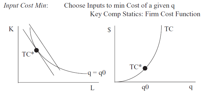 Figure 14.1: Initial cost minimization and cost function.
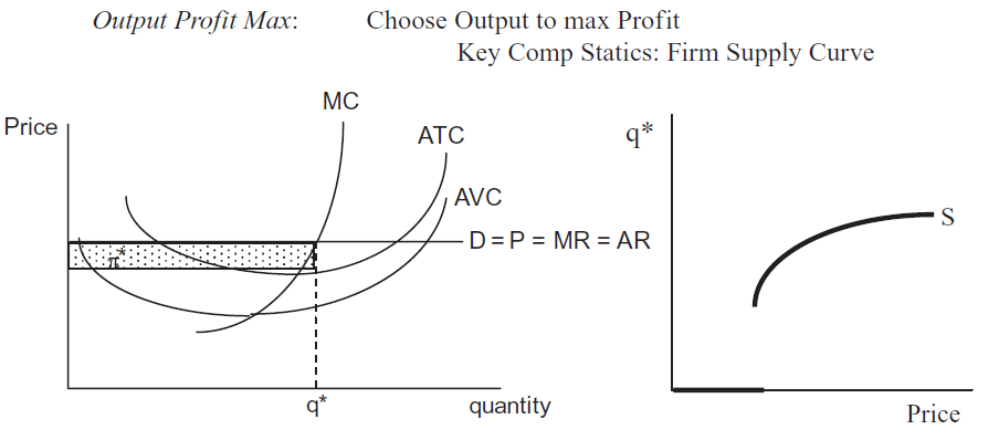 Figure 14.2: Initial profit maximization and the supply curve.
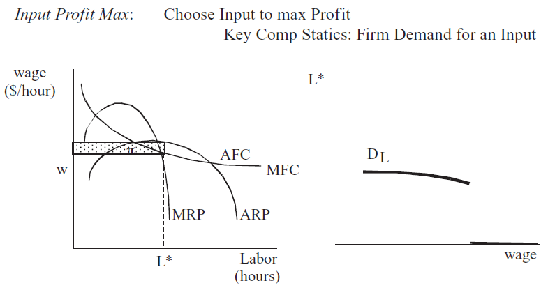 Figure 14.3: Initial profit maximization and the demand for labor.
 button to fit the graphs on your screen so that all of them can be seen simultaneously.
 button, and then implement a labor productivity increase to 0.751 by changing cell F2.
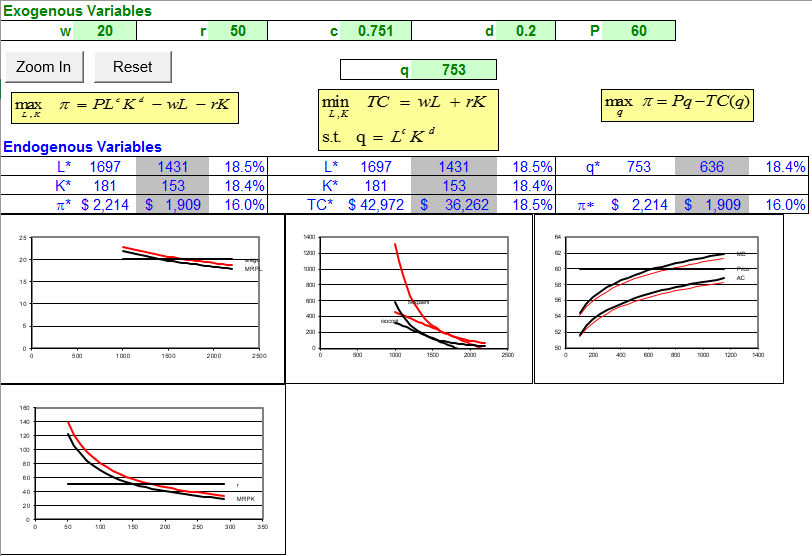
 button if needed to see more clearly how the graphs have changed.
 button, then implement a labor productivity increase to 0.751 by changing cell F2.