In perfect competition, firms are price takers with no power to affect the market price. Each firm optimizes by choosing q to equalize MC and P.
In monopoly, the sole seller of a product with no close substitutes optimizes by choosing q to equalize MC and MR and then charges the highest price that clears the market (given by the demand curve).
In both market structures, the profits of the individual firm are not affected by what anyone else does. In perfect competition, there are so many other firms that Firm i does not care about what Firm j is doing. In monopoly, there is no other firm to worry about.
What about market structures between the extremes of perfect competition and monopoly? Oligopoly is a market dominated by a few firms. Their decisions are interdependent. In other words, what each individual firm chooses does affect the sales and profits of the other firm. To optimize, each firm must anticipate what their rivals will do and then choose its best options. This is clearly a more realistic model than that of perfect competition and monopoly, which rely on idealized, abstract descriptions of firms that have no real-world counterparts.
How do oligopolies behave? We know that, like other firms, they optimize given the economic environment, but because of interdependence, it is much more difficult to analyze.
This chapter opens the door to the analysis of strategic behavior. It presents a few basic ideas from the fields of Game Theory and Industrial Organization.
Interdependence and Nash Equilibrium
It seems obvious when we say that firms are interdependent, but exactly what does this mean? Consider two power companies that generate and sell electricity. This is a good example of a homogeneous product. We assume consumers do not care at all which of the two firms provides electricity to their homes.
To keep it simple, suppose that each power company can choose either a high level of output or a low level of output. Market price is a function of the output decisions of the two firms. Each power company’s profits are functions of their own decision to produce and the market price.
Figure 16.1 displays a payoff matrix, which shows the possible choices and outcomes. You read the entries in the payoff matrix like coordinate pairs on a graph, the first part is for Firm 1 and the second for Firm 2. The $300, $300 pair in the top left of the four entries says that Firm 1 chose high output and Firm 2 chose high output. Each firm ends up with low profits.
Figure 16.1: The payoff matrix.
If Firm 2 had chosen low output (top right), Firm 1 profits would be much higher, $1,000, because it made a lot of output and price rose when Firm 2 decided to cut back.
This particular game is a one-shot, simultaneous-move game known as the Prisoner’s Dilemma. You have probably seen it before. Two criminals are arrested and questioned separately. If both stay silent, they get 1 year in jail. If both confess, they get 3 years. But if one confesses and the other does not, the one who talks gets no jail time and the silent one gets 10 years.
You can match those outcomes to the payoff matrix in Figure 16.1. The outcome that is best for both firms together is $1600 total, with $800 for each company. But, like the criminals version of the game, that is going to be an unlikely outcome. Suppose that both agree beforehand that they are going to collude and both choose low output. Unless they can write a binding agreement that is enforceable (so a cheater can be punished), there is an incentive for each firm to change its decision and choose high output if it thinks that the other firm will stick with low output. As a result, both firms end up with low profits (and both criminals confess).
If you think the other firm is going to cheat, your best move is to also cheat. If you think the other firm is going to honor the agreement, your best move, in the sense of profit maximization, is to cheat and produce a high output (assuming this is a one-time game and you never have to see your opponent again). It looks like cheating, producing high output (or confessing), is the best move no matter what the other firm does. We say that this game has a dominant strategyproduce high output (confess).
This result illustrates the reason why cartelsgroups of firms that get together to charge the monopoly price and split the monopoly profitsare unstable. It is difficult for oligopolistic firms to get together and act like a monopoly because there is an incentive for individual firms to cheat on the agreement and produce more to take advantage of high prices.
Because of the interdependence of firms’ decision making, competition among firms in an oligopoly may resemble military operations involving tactics, strategies, moves, and countermoves. Economists model these sophisticated decision making processes using game theory, a branch of mathematics and economics that was developed by John von Neumann (pronounced noy-man) and Oskar Morgenstern in the 1930s. One of the most important contributors to game theory is John Nash, a mathematician who shared the Nobel Prize in Economics.
A game-theoretic analysis of oligopoly is based on the assumption that each firm assumes that its rivals are optimizing agents. That is, managers act as though their opponents or rivals will always adopt the most profitable countermove to any move they make. The manager’s job is to find the optimal response.
Nash’s most important and enduring contribution is the concept named after him, the Nash equilibrium. Once we are in a world where firms are interdependent and one firm’s profits depends on what other firms do, we are out of the world of exogenously given price that we used for perfect competition and out of the isolated world of the monopolist. John Nash invented an equilibrium concept that describes a state of rest in this new world of interdependence.
A Nash equilibrium exists when each player, observing what her rivals have chosen, would not choose to alter the move she herself chose. In other words, this is a no regrets equilibrium: After observing the outcome, the player does not wish she would have done something else instead.
We will explore in detail a concrete example of a duopoly (a market with two firms) with a single Nash equilibrium. Remember, however, that this is simply one example. Some games have one Nash equilibrium, some have many, and some have none. There are many, many games and scenarios in game theory and we will look at just one simple example.
The Cournot Model
Augustin Cournot (pronounced coor-no) was a remarkably creative 19th-century French economist (see the References in section 12.2). Cournot originally set up a model of duopolists who produce the same good and optimize by choosing their own output levels based on assumptions about what the rival will do.
Here is the set up:
Two firms.
Each produces the exact same product.
Constant unit cost.
Firms choose output levels at the same time.
Both know the market demand for the product.
The profit of each firm depends on how much it produces and how much its rival produces. If the rival produces a lot, the the market price falls. The interdependence is that one firm’s decision about how much to produce affects the price and, thus, the rival’s profit.
What strategy should each firm use to choose its output level? The answer depends on its beliefs regarding its rival’s behavior.
STEP Open the Excel workbook GameTheory.xls and read the Intro sheet, then go to the Parameters sheet.
Market demand is given by the linear inverse demand curve and, for simplicity, we assume a linear total cost function. This means that \(MC = AC\) is a horizontal line.
STEP Proceed to the PerfectCompetition sheet.
With many small PC firms, the industry as a whole will produce where demand intersects supply (which is the sum of the individual firm’s MCs). The graph shows that a perfectly competitive market will produce 15,000 kwh at a price of 5/kwh.
What happens if a single firm takes over the entire market?
STEP Proceed to the Monopoly sheet. Use the Choose Q slider control to determine the profit-maximizing quantity. Keep your eye on cell B18 as you adjust output. The optimal output is found where \(MR = MC\).
The monopolist will produce 7500 kwh and charge a price of 12.5/kwh. This solution nets a maximum profit of 56,250 cents.
Not surprisingly, compared to the perfectly competitive results, monopoly results in lower output and higher prices.
Cournot was the first to ask the question, "What happens if the industry is shared by two firms?"
To understand the answer, the concept of residual demand is crucial because it enables us to solve the firm’s optimization problem. Residual demand is the demand curve facing the firm after the sales from the other firm are subtracted. From there, the reaction function for each firm is derived from a comparative statics analysis. The two reaction functions are then combined to yield the Nash equilibrium, which is the answer to Cournot’s question. That is confusing. We turn to Excel to see each step and how it all works.
Residual Demand
To figure out the quantity and price combination with two competing firms, we need to understand how the firms will behave.
STEP Proceed to the ResidualDemand sheet.
This sheet shows how Firm 1 decides what to do, given Firm 2’s output decision. Think of the chart as belonging to Firm 1. It will use this chart to decide what to do, given different scenarios.
Conjectured Q2, in cell B14, is the key variable. A conjecture is an educated guess. It is based on incomplete information. Firm 1 does not know and cannot control what Firm 2 is going to do. Firm 1 must act, however, so it treats Firm 2’s output decision as a conjecture and proceeds based on that projected value.
Conjectured Q2 is an exogenous variable for Firm 1. It does not know what Firm 2 will do and cannot control it. The conjectured output of Firm 2 may be different from Firm 2’s actual output. Firm 1 can, however, examine how it would react to different possible values of Firm 2 output.
The ResidualDemand sheet opens with Conjectured Q2 = 0. In this scenario, Firm 2 produces nothing and Firm 1 behaves as a monopolist, producing 7,500 kwh and charging a price of 12.5/kwh.
STEP Click five times on the scroll bar in cell C14. With each click, Conjectured Q2 rises by 1,000 units and the red lines in the graph shift left.
The red lines are the critical factor for Firm 1. They represent residual demand and residual marginal revenue. The idea behind residual demand is that Firm 2’s output will be sold first, leaving Firm 1 with the rest of the market.
The residual in the name refers to the fact that Firm 2 will supply a given amount of the market and then Firm 1 is free to decide what to do with the demand that is left over.
With each click, Firm 2 was producing more and so the demand left over for Firm 1 was falling. This is why the residual demand shifts left when Firm 2 produces more.
As the Parameters sheet shows, the inverse demand curve for the entire market is given by the function \(P = 20 - 0.001Q\). If Conjectured Q2 = 5,000, then the residual inverse demand curve is \(P = 20 - 0.001Q - 0.001(5000)\). In other words, we subtract the amount supplied by Firm 2. Thus, the residual inverse demand curve is \(P = 15 - 0.001Q\).
Figure 16.2 shows how the residual demand is shifted left by 5,000 kwh when Conjectured Q2 is 5,000. The key idea is that Firm 2’s output is subtracted from the demand curve and what is left over, the residual, is the demand faced by Firm 1.
Figure 16.2: Residual demand.
Source: GameTheory.xls!ResidualDemand
Once we have residual demand for Firm 1, we can find the profit-maximizing solution. Firm 1 derives residual MR from its residual demand curve and uses this to maximize profits by setting residual \(MR = MC\). In Figure 16.2, Firm 1 is not maximizing profits by producing 7,500 units and charging 7.5/kwh. Notice that the price is read from the residual demand curve, not the full market demand curve.
STEP Use the scroll bar (below the chart) to find Firm 1s optimal solution when Conjectured Q2 is 5,000.
You should have found that optimal \(Q\) is 5,000 kwh, optimal P = 10/kwh and maximum \(\pi\) are 25,000 cents.
The Reaction Function
Now that we know how the duopolist uses residual demand to choose the quantity (and price) that maximizes profits, we can proceed to the next step in answering Cournot’s question: "What happens if the industry is shared by two firms?"
We track each duopolist’s optimal output as a function of Conjectured Q2. This gives the reaction (or best response) function. The reaction function is a comparative statics analysis based on shocking Conjectured Q2.
STEP Fill in the table in the Residual Demand sheet. You are picking points off of Firm 1’s reaction function.
You already have two of the rows. In addition to the optimal solution at Conjectured Q2 = 5,000 which we just found, when Conjectured Q2 = 0, optimal output is 7,500 and optimal price is 12.5/kwh. Fill in the rest of the table.
STEP Check your work by clicking the button.
The filled in table is giving us Firm 1’s reaction function. It is similar to the output of the CSWizthe leftmost column is the exogenous variable and the other columns are endogenous responses.
Deriving Firm 1’s reaction function is an important step in figuring out how two firms will interact. The reaction function gives us Firm 1’s optimal response to Firm 2’s output decision. We do not know, however, what Firm 2 will actually do. It has a reaction function just like Firm 1. The two firms must interact to determine what will happen in the market.
Finding the Nash Equilibrium
Residual demand enabled us to understand the reaction function. We are now ready for the third and final step so we can answer Cournot’s question concerning the results of a duopoly. Remember, perfect competition gives 15,000 kwh of output and monopoly gives only 7,500 (and at a higher price). Presumably, duopoly is between them, but where?
STEP Proceed to the Duopoly sheet.
The display is new, but easy to understand. Instead of working with just Firm 1, both are shown. They have the same costs.
The sheet has buttons that make it a snap to see what each firm will do. The analytical solution is used so you do not have to run Solver every time Conjectured Q2 changes.
STEP Notice that Conjectured Q2 (in cell B13) is zero. To find the optimal solution, click the button.
Not surprisingly (given our earlier work with the residual demand graph) since Conjectured Q2 is zero, Firm 1 chooses to produce 7500 kwh.
But look at cell G13Firm 1 has optimized, but now we need to ask what Firm 2 would do if Firm 1 made 7,500 kwh? Firm 2 wants to maximize profits just like Firm 1.
STEP Click the button.
Firm 2’s solution makes sense. If Firm 1 makes 7,500 kwh, then Firm 2 maximizes profits by taking the residual demand and producing 3,750 kwh. Their combined output means \(P=8.75\).
This is not, however, an equilibrium solution because Firm 1 is not going to produce 7,500 kwh. Why not?
STEP Look at cell B13. Click on cell B13.
B13’s formula, =G20, makes clear how Firm 1’s decision is connected to its rival. If Firm 2 says it wants to produce 3,750, then Firm 1 regrets and will change its previous choice. We need to find the optimal output for Firm 1 given Firm 2’s new level of output.
STEP Click the button.
Firm 1 chooses to make 5,625 kwh (based on Firm 2’s output of 3,750 kwh), but now we return to Firm 2. Will it produce 3,750 kwh? No. When Firm 1 changed its output, cell G13 updated. Like B13, G13 connects Firm 2’s optimal decision to Firm 1’s output choice.
It is Firm 2’s turn to regret its previous decision. Firm 2 can make higher profits by changing its output when Firm 1 makes 5,625 kwh. How much will Firm 2 want to produce? Let’s find out.
STEP Click the button.
Firm 2 is set, but what about Firm 1? Does it regret making 5,625? Yes, it does because it can make higher profits by changing its decision.
We will not be in equilibrium until both firms are happy with their output choice and do not wish to change it. Since Firm 2 changed its output, Firm 1 will want to change its output.
STEP Click the button.
You might be thinking that this will never end. That is incorrect. It will end. You can actually see it end.
STEP Repeatedly move back and forth, clicking the and buttons, one after the other. What happens?
After repeatedly clicking, you are looking at convergence. Clearly, the two optimal output levels closed in on 5,000this is the Nash equilibrium solution to this problem and the answer to Cournot’s question. The duopoly will produce a combined total of 10,000 kwh with a price of 10/kwh. This makes sense since it is in between the perfectly competitive (15,000 kwh) and monopoly outcomes (7,500 kwh).
Manually optimizing for each firm in turn, back and forth, until the equilibrium solutions comes into focus is a great way to understand the concept of a Nash equilibrium. It is a position of rest where neither firm regrets its previous decision. In fact, a Nash equilibrium is often referred to as a "no regrets" point. There is, however, a faster way to find the position of rest.
STEP click the button.
This button does all of the hard work for you. It alternately solves one firm’s problem given the other firm’s output many times. It continues to maximize firm profits until there is less than a 0.001 difference between a firm’s optimal output and its optimal output based on the conjectured output of its rival.
STEP To see this, click on cells B20 and G20. They are close to 5,000, but not exactly 5,000.
The button also displays the individual firm’s reaction functions (scroll down if needed). In this case, the two reaction functions are identical.
Finally, the button shows the two reaction functions on the same chart and the intersection instantly reveals the Nash equilibrium. Figure 16.3 shows the Nash equilibrium chart with additional elements to help explain it.
Figure 16.3: Nash equilibrium.
Source: GameTheory.xls!Duopoly
Point 1 in Figure 16.3 represents the first time Firm 1 maximized profits, with Conjectured Q2 of zero. Point 2 shows Firm 2’s optimization based on Firm 1 making 7,500 kwh. You can see, by following the arrows, how this would lead to the intersection as the Nash equilibrium.
You might wonder why the reaction functions are not the same in Figure 16.3 since they are identical when graphed by themselves (as shown below the buttons in the Duopoly sheet). The answer lies in the axesto plot them both on the same graph, we use the reaction function for Firm 2 and the inverse reaction function for Firm 1. Scroll down to see the inverse reaction function starting in row 63.
Remember: A Nash equilibrium exists when each player, observing what her rivals have chosen, would not choose to alter the move she herself chose. Nash equilibrium is a no regrets point for all players.
Figure 16.3 shows that the Nash equilibrium is at the intersection of the two reaction functions. Only there will both firms decline the offer to change their optimal decisions. This is a position of rest.
Evaluating Duopoly’s Nash Equilibrium
We know the answer to Cournot’s question. Duopoly, at its Nash equilibrium, leaves us in between perfect competition and monopoly. But we can say more about the duopoly outcome. We focus on profits.
STEP In cell D16 in the Duopoly sheet, enter a formula that adds the profits of the two firms at the Nash equilibrium. What are industry profits?
You might recall monopoly had maximum profits of 56,250 cents. That is better than the 50,000 cents you just computed with your formula in cell D16 of = B16 + G16.
Can duopolists increase their profits to 56,250 like a monopolist? Yes, they can, but they will not be able to honor their commitments.
STEP Set quantities for both firms (in cells B20 and G20) to 3,750. What happens to profits?
Amazingly, they go up. If the two rivals can agree to simply split the monopoly output of 7,500 kwh, each will make 28,125 cents and match the monopoly outcome.
But this will not last. Why not? Why don’t the two firms get together and produce 3,750 units each and make greater joint profits than the Nash equilibrium solution? A single click reveals the answer.
STEP Click the button or the button.
If the rival makes 3,750 kwh, the firm maximizes profits at 5,625 kwh. In other words, they have an incentive to cheatjust like in the Prisoner’s Dilemma game.
As soon as one takes advantage, the other fires back and they spin back to the Nash equilibrium.
You might suggest writing a contract, but that is illegal and unenforceable in the United States. There are other options and strategies, but they would take us too far from Intermediate Microeconomics. One strong attraction that is easy to see is merger. If the two firms combine into a single entity, they will be a monopoly and enjoy monopoly profits. Presumably, the Department of Justice would object.
Interdependence
Game theory is an exciting, growing area of economics. Its primary appeal lies in the realistic modeling of agents as strategic decision makers playing against each other, moving and countering. This is obviously what a real-world firm does.
The Cournot model is a simple game matching two firms against each other. It illustrates nicely the notion of interdependence and how one firm moves, and then the other responds, and so on. Whereas some games do not have a Nash equilibrium, the Cournot duopolists do settle down to a position of rest.
The Summary sheet has the outcomes from perfect competition, duopoly, and monopoly. It is clear that monopoly maximizes firm profits, but perfect competition offers the consumer the lowest price and most output. We will return to this comparison in the third and final part of this book.
We have just scratched the surface of game theory. There are many, many more games. The workbook RockPaperScissors.xls lets you play this child’s game in Excel. Section 17.7 on Cartels and Deadweight Loss has another application of game theory.
For an entertaining version of the Prisoner’s Dilemma in a game show, see this Golden Balls episode finale: tiny.cc/splitsteal. And for a really clever twist, watch this one: tiny.cc/ibrahim. Nick’s strategy has been outlawed from the show. The Cornell game theory blog has an entry explaining it: tiny.cc/splitstealanalysis.
Exercises
These exercises are based on \(c_1=5\). If you did the Q&A questions and changed this parameter, change it back to its original value.
If Conjectured Q2 is 15,000, why does Firm 1 decide to produce nothing? Use the ResidualDemand sheet to support your explanation.
Suppose Firm 1 produces 4,500 kwh and Firm 2 produces 6,000 kwh. Does Firm 1 have any regrets? Does Firm 2 have any regrets? Enter these two values in the Duopoly sheet and click the buttons. Which firm changed its mind? Why?
Click the button in the Duopoly sheet. Explore the effect of changing Firm 1’s cost function so that \(c_2\) (cell B10) is 0.001 (with B11 = 5). How does this affect the Nash equilibrium?
References
The epigraph is from page 75 of Sylvia Nasar, A Beautiful Mind (1998). This biography of Nash has won countless awards and was made into an Academy Award-winning motion picture, with Russell Crowe starring as John Nash. Although much of the book is devoted to Nash’s personal struggle with schizophrenia, Nasar’s book gives a clear and engaging review of game-theoretic concepts before Nash and of the Nash equilibrium.
On the game Nash invented that is mentioned in the epigraph, Nasar writes,
That spring, Nash astounded everyone by inventing an extremely clever game that quickly took over the common room. Piet Hein, a Dane, had invented the game a few years before Nash, and it would be marketed by Parker Brothers in the mid-1950s as Hex. But Nash’s invention of the game appears to have been entirely independent. (p. 76)


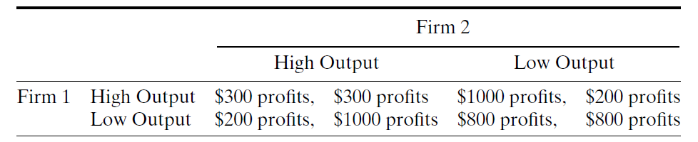 Figure 16.1: The payoff matrix.
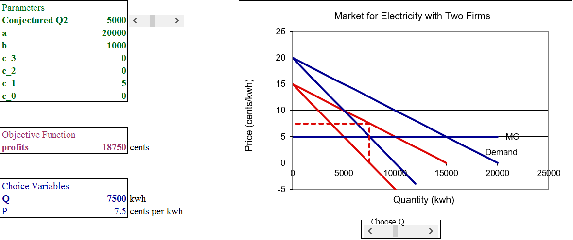
 button.
 button.
 button.
 button.
 button.
 button.
 and
and  buttons, one after the other. What happens?
 button.
 button also displays the individual firm’s reaction functions (scroll down if needed). In this case, the two reaction functions are identical.
 button shows the two reaction functions on the same chart and the intersection instantly reveals the Nash equilibrium. Figure 16.3 shows the Nash equilibrium chart with additional elements to help explain it.
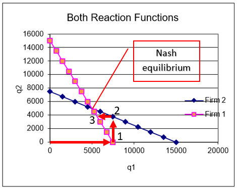
 button or the
  button.
 buttons. Which firm changed its mind? Why?
 button in the Duopoly sheet. Explore the effect of changing Firm 1’s cost function so that \(c_2\) (cell B10) is 0.001 (with B11 = 5). How does this affect the Nash equilibrium?