Market Differences Between Monopoly and Perfect Competition
Monopolies, as opposed to perfectly competitive markets, have high barriers to entry and a single producer that acts as a price maker.
learning objectives
- Distinguish between monopolies and competitive firms
A market can be structured differently depending on the characteristics of competition within that market. At one extreme is perfect competition. In a perfectly competitive market, there are many producers and consumers, no barriers to enter and exit the market, perfectly homogeneous goods, perfect information, and well-defined property rights. This produces a system in which no individual economic actor can affect the price of a good – in other words, producers are price takers that can choose how much to produce, but not the price at which they can sell their output. In reality there are few industries that are truly perfectly competitive, but some come very close. For example, commodity markets (such as coal or copper) typically have many buyers and multiple sellers. There are few differences in quality between providers so goods can be easily substituted, and the goods are simple enough that both buyers and sellers have full information about the transaction. It is unlikely that a copper producer could raise their prices above the market rate and still find a buyer for their product, so sellers are price takers.
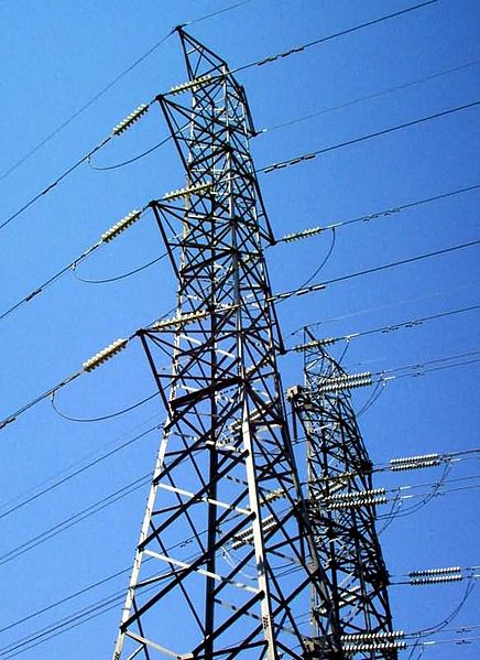
A monopoly, on the other hand, exists when there is only one producer and many consumers. Monopolies are characterized by a lack of economic competition to produce the good or service and a lack of viable substitute goods. As a result, the single producer has control over the price of a good – in other words, the producer is a price maker that can determine the price level by deciding what quantity of a good to produce. Public utility companies tend to be monopolies. In the case of electricity distribution, for example, the cost to put up power lines is so high it is inefficient to have more than one provider. There are no good substitutes for electricity delivery so consumers have few options. If the electricity distributor decided to raise their prices it is likely that most consumers would continue to purchase electricity, so the seller is a price maker.

Electricity Distribution: The cost of electrical infrastructure is so expensive that there are few or no competitors for electricity distribution. This creates a monopoly.
Sources of Monopoly Power
Monopoly power comes from markets that have high barriers to entry. This can be caused by a variety of factors:
- Increasing returns to scale over a large range of production
- High capital requirements or large research and development costs
- Production requires control over natural resources
- Legal or regulatory barriers to entry
- The presence of a network externality – that is, the use of a product by a person increases the value of that product for other people
Monopoly Vs. Perfect Competition
Monopoly and perfect competition mark the two extremes of market structures, but there are some similarities between firms in a perfectly competitive market and monopoly firms. Both face the same cost and production functions, and both seek to maximize profit. The shutdown decisions are the same, and both are assumed to have perfectly competitive factors markets.
However, there are several key distinctions. In a perfectly competitive market, price equals marginal cost and firms earn an economic profit of zero. In a monopoly, the price is set above marginal cost and the firm earns a positive economic profit. Perfect competition produces an equilibrium in which the price and quantity of a good is economically efficient. Monopolies produce an equilibrium at which the price of a good is higher, and the quantity lower, than is economically efficient. For this reason, governments often seek to regulate monopolies and encourage increased competition.
Marginal Revenue and Marginal Cost Relationship for Monopoly Production
For monopolies, marginal cost curves are upward sloping and marginal revenues are downward sloping.
learning objectives
- Analyze how marginal and marginal costs affect a company’s production decision
Profit Maximization
In traditional economics, the goal of a firm is to maximize their profits. This means they want to maximize the difference between their earnings, i.e. revenue, and their spending, i.e. costs. To find the profit maximizing point, firms look at marginal revenue (MR) – the total additional revenue from selling one additional unit of output – and the marginal cost (MC) – the total additional cost of producing one additional unit of output. When the marginal revenue of selling a good is greater than the marginal cost of producing it, firms are making a profit on that product. This leads directly into the marginal decision rule, which dictates that a given good should continue to be produced if the marginal revenue of one unit is greater than its marginal cost. Therefore, the maximizing solution involves setting marginal revenue equal to marginal cost.
This is relatively straightforward for firms in perfectly competitive markets, in which marginal revenue is the same as price. Monopoly production, however, is complicated by the fact that monopolies have demand curves and MR curves that are distinct, causing price to differ from marginal revenue.

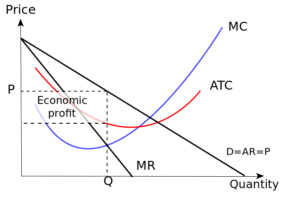
Monopoly: In a monopoly market, the marginal revenue curve and the demand curve are distinct and downward-sloping. Production occurs where marginal cost and marginal revenue intersect.

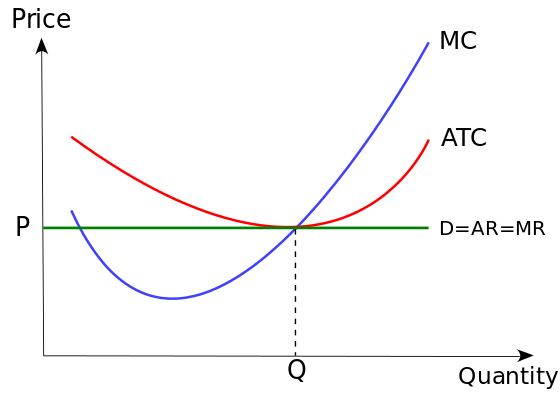
Perfect Competition: In a perfectly competitive market, the marginal revenue curve is horizontal and equal to demand, or price. Production occurs where marginal cost and marginal revenue intersect.
Monopoly Profit Maximization
The marginal cost curves faced by monopolies are similar to those faced by perfectly competitive firms. Most will have low marginal costs at low levels of production, reflecting the fact that firms can take advantage of efficiency opportunities as they begin to grow. Marginal costs get higher as output increases. For example, a pizza restaurant can easily double production from one pizza per hour to two without hiring additional employees or buying more sophisticated equipment. When production reaches 50 pizzas per hour, however, it may be difficult to grow without investing a lot of money in more skilled employees or more high-tech ovens. This trend is reflected in the upward-sloping portion of the marginal cost curve.
The marginal revenue curve for monopolies, however, is quite different than the marginal revenue curve for competitive firms. While competitive firms experience marginal revenue that is equal to price – represented graphically by a horizontal line – monopolies have downward-sloping marginal revenue curves that are different than the good’s price.
Profit Maximization Function for Monopolies
Monopolies set marginal cost equal to marginal revenue in order to maximize profit.
learning objectives
- Explain the monopolist’s profit maximization function
Monopolies have much more power than firms normally would in competitive markets, but they still face limits determined by demand for a product. Higher prices (except under the most extreme conditions) mean lower sales. Therefore, monopolies must make a decision about where to set their price and the quantity of their supply to maximize profits. They can either choose their price, or they can choose the quantity that they will produce and allow market demand to set the price.
Since costs are a function of quantity, the formula for profit maximization is written in terms of quantity rather than in price. The monopoly’s profits are given by the following equation:
\[π=p(q)q−c(q)\]
In this formula, p(q) is the price level at quantity q. The cost to the firm at quantity q is equal to c(q). Profits are represented by π. Since revenue is represented by pq and cost is c, profit is the difference between these two numbers. As a result, the first-order condition for maximizing profits at quantity q is represented by:
\[0=∂q=p(q)+qp′(q)−c′(q)\]
The above first-order condition must always be true if the firm is maximizing its profit – that is, if \(p(q)+qp′(q)−c′(q)\) is not equal to zero, then the firm can change its price or quantity and make more profit.
Marginal revenue is calculated by \(p(q)+qp′(q)\), which is derived from the term for revenue, \(pq\). The term \(c′(q)\) is marginal cost, which is the derivative of c(q). Monopolies will produce at quantity q where marginal revenue equals marginal cost. Then they will charge the maximum price \(p(q)\) that market demand will respond to at that quantity.
Consider the example of a monopoly firm that can produce widgets at a cost given by the following function:
\[c(q)=2+3q+q^2\]
If the firm produces two widgets, for example, the total cost is \(2+3(2)+2^2=12\). The price of widgets is determined by demand:
\[p(q)=24-2p\]
When the firm produces two widgets it can charge a price of \(24-2(2)=20\) for each widget. The firm’s profit, as shown above, is equal to the difference between the quantity produces multiplied by the price, and the total cost of production: \(p(q)q−c(q)\). How can we maximize this function?
Using the first order condition, we know that when profit is maximized, \(0=p(q)+qp′(q)−c′(q)\). In this case:
\[0=(24-2p)+q(-2)-(3+2q)=21-6q\]
Rearranging the equation shows that \(q=3.5\). This is the profit maximizing quantity of production.
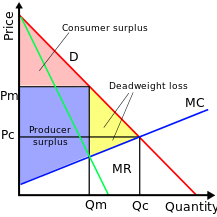
Consider the diagram illustrating monopoly competition. The key points of this diagram are fivefold.
- First, marginal revenue lies below the demand curve. This occurs because marginal revenue is the demand, p(q), plus a negative number.
- Second, the monopoly quantity equates marginal revenue and marginal cost, but the monopoly price is higher than the marginal cost.
- Third, there is a deadweight loss, for the same reason that taxes create a deadweight loss: The higher price of the monopoly prevents some units from being traded that are valued more highly than they cost.
- Fourth, the monopoly profits from the increase in price, and the monopoly profit is illustrated.
- Fifth, since—under competitive conditions—supply equals marginal cost, the intersection of marginal cost and demand corresponds to the competitive outcome.
We see that the monopoly restricts output and charges a higher price than would prevail under competition.

Monopoly Diagram: This graph illustrates the price and quantity of the market equilibrium under a monopoly.
Monopoly Production Decision
To maximize output, monopolies produce the quantity at which marginal supply is equal to marginal cost.
learning objectives
- Explain how to identify the monopolist’s production point
Monopoly Production
A pure monopoly has the same economic goal of perfectly competitive companies – to maximize profit. If we assume increasing marginal costs and exogenous input prices, the optimal decision for all firms is to equate the marginal cost and marginal revenue of production. Nonetheless, a pure monopoly can – unlike a firm in a competitive market – alter the market price for its own convenience: a decrease of production results in a higher price. Because of this, rather than finding the point where the marginal cost curve intersects a horizontal marginal revenue curve (which is equivalent to good’s price), we must find the point where the marginal cost curve intersect a downward-sloping marginal revenue curve.
Monopoly Production Point
Like non-monopolies, monopolists will produce the at the quantity such that marginal revenue (MR) equals marginal cost (MC). However, monopolists have the ability to change the market price based on the amount they produce since they are the only source of products in the market. When a monopolist produces the quantity determined by the intersection of MR and MC, it can charge the price determined by the market demand curve at the quantity. Therefore, monopolists produce less but charge more than a firm in a competitive market.

Monopoly Production: Monopolies produce at the point where marginal revenue equals marginal costs, but charge the price expressed on the market demand curve for that quantity of production.
In short, three steps can determine a monopoly firm’s profit-maximizing price and output:
- Calculate and graph the firm’s marginal revenue, marginal cost, and demand curves
- Identify the point at which the marginal revenue and marginal cost curves intersect and determine the level of output at that point
- Use the demand curve to find the price that can be charged at that level of output
Monopoly Price and Profit
Monopolies can influence a good’s price by changing output levels, which allows them to make an economic profit.
learning objectives
- Analyze the final price and resulting profit for a monopolist
Monopolies, unlike perfectly competitive firms, are able to influence the price of a good and are able to make a positive economic profit. While a perfectly competitive firm faces a single market price, represented by a horizontal demand/marginal revenue curve, a monopoly has the market all to itself and faces the downward-sloping market demand curve. An important consequence is worth noticing: typically a monopoly selects a higher price and lesser quantity of output than a price-taking company; again, less is available at a higher price.
Imagine that the market demand for widgets is \(Q=30-2P\). This says that when the price is one, the market will demand 28 widgets; when the price is two, the market will demand 26 widgets; and so on. The monopoly’s total revenue is equal to the price of the widget multiplied by the quantity sold: \(P(30-2P)\). This can also be rearranged so that it is written in terms of quantity: total revenue equals \(Q(30-Q)/2\).
The firm can produce widgets at a total cost of \(2Q^2\), that is, it can produce one widget for $2, two widgets for $8, three widgets for $18, and so on. We know that all firms maximize profit by setting marginal costs equal to marginal revenue. Finding this point requires taking the derivative of total revenue and total cost in terms of quantity and setting the two derivatives equal to each other. In this case:
\[\dfrac{dTR}{dQ}=\dfrac{(30−2Q)}{2}\]
\[\dfrac{dTC}{dQ}=4Q\]
Setting these equal to each other: \(15−Q=4Q\)
So the profit maximizing point occurs when \(Q=3\).
At this point, the price of widgets is $13.50, the monopoly’s total revenue is $40.50, the total cost is $18, and profit is $22.50. For comparison, it is easy to see that if the firm produced two widgets price would be $14 and profit would be $20; if it produced four widgets price would be $13 and profit would again be $20. Q=3 must be the profit-maximizing output for the monopoly.
Graphically, one can find a monopoly’s price, output, and profit by examining the demand, marginal cost, and marginal revenue curves. Again, the firm will always set output at a level at which marginal cost equals marginal revenue, so the quantity is found where these two curves intersect. Price, however, is determined by the demand for the good when that quantity is produced. Because a monopoly’s marginal revenue is always below the demand curve, the price will always be above the marginal cost at equilibrium, providing the firm with an economic profit.

Monopoly Pricing: Monopolies create prices that are higher, and output that is lower, than perfectly competitive firms. This causes economic inefficiency.
Key Points
- In a perfectly competitive market, there are many producers and consumers, no barriers to exit and entry into the market, perfectly homogenous goods, perfect information, and well-defined property rights.
- Perfectly competitive producers are price takers that can choose how much to produce, but not the price at which they can sell their output.
- A monopoly exists when there is only one producer and many consumers.
- Monopolies are characterized by a lack of economic competition to produce the good or service and a lack of viable substitute goods.
- Firm typically have marginal costs that are low at low levels of production but that increase at higher levels of production.
- While competitive firms experience marginal revenue that is equal to price – represented graphically by a horizontal line – monopolies have downward-sloping marginal revenue curves that are different than the good’s price.
- For monopolies, marginal revenue is always less than price.
- The first-order condition for maximizing profits in a monopoly is 0=∂q=p(q)+qp′(q)−c′(q), where q = the profit-maximizing quantity.
- A monopoly’s profits are represented by π=p(q)q−c(q), where revenue = pq and cost = c.
- Monopolies have the ability to limit output, thus charging a higher price than would be possible in competitive markets.
- Unlike a competitive company, a monopoly can decrease production in order to charge a higher price.
- Because of this, rather than finding the point where the marginal cost curve intersects a horizontal marginal revenue curve (which is equivalent to good’s price), we must find the point where the marginal cost curve intersect a downward-sloping marginal revenue curve.
- Monopolies have downward sloping demand curves and downward sloping marginal revenue curves that have the same y-intercept as demand but which are twice as steep.
- The shape of the curves shows that marginal revenue will always be below demand.
- Typically a monopoly selects a higher price and lesser quantity of output than a price-taking company.
- A monopoly, unlike a perfectly competitive firm, has the market all to itself and faces the downward-sloping market demand curve.
- Graphically, one can find a monopoly’s price, output, and profit by examining the demand, marginal cost, and marginal revenue curves.
Key Terms
- perfect competition: A type of market with many consumers and producers, all of whom are price takers
- network externality: The effect that one user of a good or service has on the value of that product to other people
- perfect information: The assumption that all consumers know all things, about all products, at all times, and therefore always make the best decision regarding purchase.
- marginal revenue: The additional profit that will be generated by increasing product sales by one unit.
- marginal cost: The increase in cost that accompanies a unit increase in output; the partial derivative of the cost function with respect to output. Additional cost associated with producing one more unit of output.
- first-order condition: A mathematical relationship that is necessary for a quantity to be maximized or minimized.
- deadweight loss: A loss of economic efficiency that can occur when an equilibrium is not Pareto optimal.
- economic profit: The difference between the total revenue received by the firm from its sales and the total opportunity costs of all the resources used by the firm.
- demand: The desire to purchase goods and services.
LICENSES AND ATTRIBUTIONS
CC LICENSED CONTENT, SPECIFIC ATTRIBUTION
- Monopoly. Provided by: Wikipedia. Located at: en.Wikipedia.org/wiki/Monopoly. License: CC BY-SA: Attribution-ShareAlike
- perfect information. Provided by: Wikipedia. Located at: en.Wikipedia.org/wiki/perfect%20information. License: CC BY-SA: Attribution-ShareAlike
- Boundless. Provided by: Boundless Learning. Located at: www.boundless.com//economics/...ct-competition. License: CC BY-SA: Attribution-ShareAlike
- network externality. Provided by: Wikipedia. Located at: en.Wikipedia.org/wiki/network%20externality. License: CC BY-SA: Attribution-ShareAlike
- Electricalgrid. Provided by: Wikipedia. Located at: en.Wikipedia.org/wiki/File:Electricalgrid.jpg. License: Public Domain: No Known Copyright
- marginal cost. Provided by: Wiktionary. Located at: en.wiktionary.org/wiki/marginal_cost. License: CC BY-SA: Attribution-ShareAlike
- marginal revenue. Provided by: Wikipedia. Located at: en.Wikipedia.org/wiki/marginal%20revenue. License: CC BY-SA: Attribution-ShareAlike
- Monopoly. Provided by: Wikipedia. Located at: en.Wikipedia.org/wiki/Monopoly. License: CC BY-SA: Attribution-ShareAlike
- Electricalgrid. Provided by: Wikipedia. Located at: en.Wikipedia.org/wiki/File:Electricalgrid.jpg. License: Public Domain: No Known Copyright
- Imperfect competition in the short run. Provided by: Wikimedia. Located at: commons.wikimedia.org/wiki/Fi..._short_run.svg. License: CC BY-SA: Attribution-ShareAlike
- Economics Perfect competition. Provided by: Wikimedia. Located at: commons.wikimedia.org/wiki/Fi...ompetition.svg. License: CC BY-SA: Attribution-ShareAlike
- Boundless. Provided by: Boundless Learning. Located at: www.boundless.com//economics/...rder-condition. License: CC BY-SA: Attribution-ShareAlike
- deadweight loss. Provided by: Wikipedia. Located at: en.Wikipedia.org/wiki/deadweight%20loss. License: CC BY-SA: Attribution-ShareAlike
- Electricalgrid. Provided by: Wikipedia. Located at: en.Wikipedia.org/wiki/File:Electricalgrid.jpg. License: Public Domain: No Known Copyright
- Imperfect competition in the short run. Provided by: Wikimedia. Located at: commons.wikimedia.org/wiki/Fi..._short_run.svg. License: CC BY-SA: Attribution-ShareAlike
- Economics Perfect competition. Provided by: Wikimedia. Located at: commons.wikimedia.org/wiki/Fi...ompetition.svg. License: CC BY-SA: Attribution-ShareAlike
- Imperfect competition in the short run. Provided by: Wikimedia. Located at: commons.wikimedia.org/wiki/Fi..._short_run.svg. License: CC BY-SA: Attribution-ShareAlike
- marginal cost. Provided by: Wiktionary. Located at: en.wiktionary.org/wiki/marginal_cost. License: CC BY-SA: Attribution-ShareAlike
- Monopoly. Provided by: Wikipedia. Located at: en.Wikipedia.org/wiki/Monopoly. License: CC BY-SA: Attribution-ShareAlike
- marginal revenue. Provided by: Wikipedia. Located at: en.Wikipedia.org/wiki/marginal%20revenue. License: CC BY-SA: Attribution-ShareAlike
- Electricalgrid. Provided by: Wikipedia. Located at: en.Wikipedia.org/wiki/File:Electricalgrid.jpg. License: Public Domain: No Known Copyright
- Imperfect competition in the short run. Provided by: Wikimedia. Located at: commons.wikimedia.org/wiki/Fi..._short_run.svg. License: CC BY-SA: Attribution-ShareAlike
- Economics Perfect competition. Provided by: Wikimedia. Located at: commons.wikimedia.org/wiki/Fi...ompetition.svg. License: CC BY-SA: Attribution-ShareAlike
- Imperfect competition in the short run. Provided by: Wikimedia. Located at: commons.wikimedia.org/wiki/Fi..._short_run.svg. License: CC BY-SA: Attribution-ShareAlike
- Imperfect competition in the short run. Provided by: Wikimedia. Located at: commons.wikimedia.org/wiki/Fi..._short_run.svg. License: CC BY-SA: Attribution-ShareAlike
- Monopoly. Provided by: Wikipedia. Located at: en.Wikipedia.org/wiki/Monopol...lasticity_rule. License: CC BY-SA: Attribution-ShareAlike
- Monopoly profit. Provided by: Wikipedia. Located at: en.Wikipedia.org/wiki/Monopoly_profit. License: CC BY-SA: Attribution-ShareAlike
- demand. Provided by: Wiktionary. Located at: en.wiktionary.org/wiki/demand. License: CC BY-SA: Attribution-ShareAlike
- Boundless. Provided by: Boundless Learning. Located at: www.boundless.com//economics/...omic-profit--2. License: CC BY-SA: Attribution-ShareAlike
- Electricalgrid. Provided by: Wikipedia. Located at: en.Wikipedia.org/wiki/File:Electricalgrid.jpg. License: Public Domain: No Known Copyright
- Imperfect competition in the short run. Provided by: Wikimedia. Located at: commons.wikimedia.org/wiki/Fi..._short_run.svg. License: CC BY-SA: Attribution-ShareAlike
- Economics Perfect competition. Provided by: Wikimedia. Located at: commons.wikimedia.org/wiki/Fi...ompetition.svg. License: CC BY-SA: Attribution-ShareAlike
- Imperfect competition in the short run. Provided by: Wikimedia. Located at: commons.wikimedia.org/wiki/Fi..._short_run.svg. License: CC BY-SA: Attribution-ShareAlike
- Imperfect competition in the short run. Provided by: Wikimedia. Located at: commons.wikimedia.org/wiki/Fi..._short_run.svg. License: CC BY-SA: Attribution-ShareAlike
- Monopoly pricing example 01. Provided by: Wikimedia. Located at: commons.wikimedia.org/wiki/Fi...example_01.svg. License: CC BY-SA: Attribution-ShareAlike


