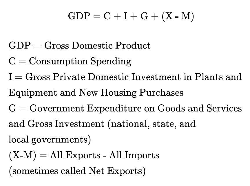
The business cycle is the term we give for the expansion and contraction of an economy. This is measured through Gross Domestic Product (GDP). GDP is the output and sale of goods and services in any economy measured over a period of time (usually one year). Traditionally, GDP is aggregated into four broad categories, as measured by the Bureau of Economic Analysis of the U.S. Commerce Department. These categories are represented in the following equation:
The largest component of GDP is Consumption Expenditure. How comfortable consumers are opening their wallets every month has an outsized effect on the GDP and the business cycle. Here is the relative value of the components of GDP for 2020 (estimated, as of June 2020) in current dollars:
C
+ $14.58 trillion
(68%)
I
+ $3.63 trillion
(17%)
G
+ $3.85 trillion
(18%)
(X-M)
– $0.53 trillion
(-2.5%)
GDP
= $21.54 trillion
(100%)
The business cycle can be visualized as a graph of the value of GDP over time. Its fluctuations from its trend line are the expansions and recessions of the economy. I show a close-up of the period from 2000 to 2016 so you can see more clearly the fluctuations in actual GDP from the trend line. The graph also includes the last two recessions, March 2001 to November 2001, and December 2007 to June 2009.
Figure 16.1. U.S. Bureau of Economic Analysis, Real Gross Domestic Product [GDPC1], retrieved from FRED, Federal Reserve Bank of St. Louis; October 1, 2021.
The blue is the trend line of GDP growing and the red is the actual real GDP. The deviation in the actual from the trend is the business cycle. The gray bars show the time of official recessions. Note that GDP is below the trend during recessions, meaning GDP has decreased. Recessions have both a popular definition and an official definition. The popular definition is a drop in economic activity (a drop in GDP) for two successive calendar quarters (six months). On the other hand, the National Bureau of Economic Research (NBER), a group of academic economists from around the U.S., is the official arbiter of when we are in a recession and when a recession is over. The NBER defines a recession as follows:
A recession is a significant decline in economic activity spread across the economy, normally visible in production, employment, and other indicators. A recession begins when the economy reaches a peak of economic activity and ends when the economy reaches its trough. Between trough and peak, the economy is in an expansion.
The terms peak and trough are an analogy to a wave on the ocean:
There have been several business cycles in the economic history of the United States. Here is a graph of GDP and recessions (in gray bars):
Figure 16.3. U.S. Bureau of Economic Analysis, Real Gross Domestic Product [GDPC1], retrieved from FRED, Federal Reserve Bank of St. Louis; October 1, 2021.
The graph covers 1940 to 2020, so the drops in GDP during recessions may look small. However, note that in the Great Recession, GDP dropped 4.1% and 8,500,000 employees lost their jobs. One the last line in the chart above, it states that since the end of WWII there have been 12 business cycles (recessions and expansions) including the Pandemic Recession. On average, recessions have lasted on average 11.1 months, while economic expansions have lasted on average 64.5 months (a little over five years).
Does this mean that we can predict recessions? If that were possible, we could all become millionaires. As you will see from the graph below, the stock market (the S&P 500 Index) drops 6 months to one year before a recession and begins trending upward again 6 months or less prior to the end of the recession. That means if we could predict a recession, we could predict the stock market.
Figure 16.4. S&P 500 1955-2020 by Fred Rowland is used under a CC BY-NC 4.0 License. Source: Yahoo Finance, 12/3/2020.
Unfortunately, the time between recessions and, to a lesser extent, the length of recessions is too variable to be able to accurately predict them. At an economic conference, I was able to ask Robert Hall, Chair of the National Bureau of Economic Research Committee on Business Cycles and professor at Stanford University, whether anyone can predict recessions. Dr. Hall said no one can predict recessions accurately. There are several characteristics of the business cycle that may not be immediately apparent from the graphs and charts above but are important to understand. Dr. Daron Acemoglu of MIT states these:
Many aggregate macroeconomic variables move together in the business cycle. In the NBER’s definition of a recession, they lay out the most important economic variables they use to determine the business cycle: “…real GDP, real income, employment, industrial production, and wholesale-retail sales” (NBER.org).
It is very hard, if not impossible, to predict the turning points in the business cycle. As I mentioned earlier, Dr. Hall said it is impossible to predict recessions. It is equally impossible to predict the turning point of a recession, when the economic expansion begins.
There is a persistence to the rate of economic growth. If the economy is growing in one quarter, it will likely grow in the next quarter as well. Contrariwise, if the economy is in a recession in one quarter, it is likely to decline again in the following quarter (Acemoglu, Laibson, & List, 2018).
There are strong psychological reasons for the persistence of the rate of economic growth. Economists today call them expectations of the future by consumers and firms. John Maynard Keynes, the father of modern economics, called these expectations animal spirits. We now call them consumer sentiment and business expectations. The fact remains that humans tend to think the near future will be a replication of the current time period and so act accordingly (this is an important tenet of Behavioral Economics.) Further, there are important economic reasons for the persistence of the rate of economic growth, mainly the circular flow of the economy:
In this simple model, there are two agents: individuals (or households) and businesses (or firms). Individuals sell their labor to businesses and receive income (wages) in return. Businesses use this labor along with factories, equipment, and raw materials (physical capital) to make goods and services. Businesses sell the goods and services to individuals who use the income they received for selling their labor to pay the businesses for the goods and services that the individuals buy (expenditures).
The circular flow of an economy contributes to the persistence of the trend of economic growth (or decline). Recessions most often begin when consumers slow down their spending on goods and services. Historically, this has been caused by a financial crisis of some sort that causes consumers to run up their debts too high. Consumers slow down their spending. The sales of businesses decline due to the decreased spending, usually first as a decline in consumer durables (Consumer durables are items that last three years or more, such as automobiles and appliances). With the decline in sales, the businesses decrease making goods and services.
Consumers buying fewer goods and services means that businesses do not need as many workers as they currently have. Because a recession is a short-term phenomenon, firms do not sell their factories and equipment; they just lay off workers. These layoffs mean a decrease in aggregate income for consumers overall, and this decreases aggregate expenditure on goods and services, leading to further layoffs. The initial drop in consumer expenditures in goods and services usually leads to further drops in consumer expenditures due to layoffs, making the recession worse. The circular flow also helps explain the persistence of economic growth. Increased purchases of goods and services by consumers results in businesses expanding production and hiring more workers. Then the increased aggregate income of consumers results in more purchases of goods and services and the hiring of more workers to make those goods and services. During these economic fluctuations, the hiring and firing of workers do not happen instantaneously, but they can happen pretty quickly and historically have always moved together. Another way of saying this is that there are lags in the co-movement of these two variables.
The Pandemic Recession was an exception to the historical start of a recession (financial crisis or excessive consumer debt) because the government-mandated COVID-19 lockdown resulted in massive layoffs of workers, especially in the hospitality industry. As you will see in the chapter on the Pandemic Recession, the U.S. government enacted a huge fiscal and monetary policy stimulus in order to counter the economic effects of the lockdown. Despite that, consumers hoarded their money, the result of consumer sentiment.
This is another example of the persistence of the rate of economic growth. When the economy is going up, it continues going up. When it is going down, it tends to continue going down. Of course, the government can do a lot of things to keep the economy rolling and a lot of things to help bring the economy out of a persistent recession.
Government Tax Policy
The government taxes us for two main reasons. The first is to run the functions of the government and provide the services, such as national security, regulation, commerce, and more. The second reason to tax us is for income redistribution through welfare payments, unemployment compensation, and aid to lower income people in the country. These payments are called transfer payments.
The government not only collects payroll taxes, it also collects corporate, social security, unemployment and other types of taxes. These are deductions from our GDP, and as such, the amount of taxes and the percent of GDP taxed influences the amount of consumer spending, corporate investment, and other aspects of the economy. This can be expressed simply:
This is true theoretically, but with a few minor adjustments, it is also true in the real world. Everything we make, we sell. The income from those sales goes to someone in the United States as income. So taxing GDP is taxing our national income, and the more the government takes, the less there is for consumers and corporations to spend. I am sad to say, though, that “the only certain things in life are death and taxes,” so taxes are here to stay. The U.S. government budget for fiscal year 2020 is below. (The government’s fiscal year 2020 runs from October 1, 2019, to September 30, 2020.) The numbers are in billions; for example, the total revenue for 2019, listed as 3,463, is $3 trillion and $463 billion.
Table 16.1. U.S. Government Budget for Fiscal Year 2020
Revenues (Billions)
2019 Actual
2020
2020 As % of 2020 GDP
Individual income taxes
1,718
1,791
Payroll taxes
1,243
1,302
Corporate income taxes
230
234
Other
271
305
Total
3,463
3,632
16.4%
On-budget
2,548
2,672
Off-budget
914
960
Outlays (Billions)
Mandatory
2,734
2,910
Discretionary
1,338
1,413
Net interest
375
383
Total
4,447
4,706
21.3%
On-budget
3,540
3,748
Off-budget
907
958
Deficit (-) or Surplus (Billions)
-984
-1,073
-4.9%
On-budget
-992
-1,075
Off-budget
8
2
Debt Held by the Public (Billions)
16,801
17,835
80.7%
Memorandum:
Gross Domestic Product
21,220
22,111
100%
Source: Congressional Budget Office, March, 2020.
Since budget numbers are changing every year and inflation is affecting our incomes and the cost of goods and services to the government, we should look at historical data so that we can evaluate whether these numbers are above or below average. Revenues and Outlays as percentages of GDP are a good benchmark. We can see those numbers in the chart below.
Table 16.2. Revenues, Outlays, Deficits (or Surpluses) and Debt Held by the Public, as a Percentage of GDP
Year
Revenues
Outlays
Deficits/ Surpluses
Debt Held by the Public
2007
18.0
19.1
-2.4
35.2
2008
17.1
20.2
-4.4
39.4
2009
14.6
24.4
-10.7
52.3
2010
14.6
23.3
-9.2
52.3
2011
15.0
23.4
-8.9
60.8
2012
15.3
22.0
-7.1
70.3
2013
16.7
20.8
-4.3
72.2
2014
17.4
20.2
-3.0
73.7
2015
18.0
20.4
-2.6
72.5
2016
17.6
20.8
-3.3
76.4
2017
17.2
20.6
-3.7
76.0
2018
16.4
20.2
-3.9
77.4
2019
16.3
21.0
-4.7
0.0
The government’s revenue as a percent of GDP (the first column in the chart above) can be considered as the average tax rate. This is because GDP is equal to Gross National Income (GNI). That is, for everything made in the United States (the GDP), the money goes to someone or some corporation in the United States. According to the table above, when the revenue of the U.S. Government as a percentage of GDP decreases (often through tax cuts) and the Outlays as a percentage of GDP do not decrease (that is, no spending cuts), you get big annual deficits.
In theory, the government budget is similar to your household budget. If you spend more than you earn, you have to borrow from your credit cards to make up the difference. If a government spends more than they take in through taxes, it must issue more Treasury Bonds to finance that deficit, and, by definition, the national debt increases.
The problem with increasing your credit card debt or a government increasing its national debt is that you each have to pay it back. You or the government must make paying down the debt a priority over spending on anything else, or your credit rating goes down. More debt decreases your ability to buy goods and services. There is a crucial difference, though; you cannot easily increase your income if you have higher debt and want to maintain your former level of spending. On the other hand, governments can raise taxes to maintain their level of spending.
Government Spending
The government’s revenues come principally from individual income taxes and payroll taxes (Social Security and Medicare tax deductions). The spending (outlays) goes to pay for (in order of size) making transfer payments, maintaining the military, and running the government. Here is a graph of the revenues and outlays of the U.S. Federal Government for 2019:
Similar to your household budget, if the government spends more than it collects in revenue, it has to borrow money to finance the deficit. In the case of the U.S., it does this by issuing more Treasury Bonds. Since the definition of the national debt is the amount of Treasury Bonds outstanding, financing the annual deficit each year with additional Treasury Bonds increases the national debt.
The graph below shows the revenues and outlays of the U.S. Government through the year 2017. The red part of each year’s bar graph represents the annual deficit. Because of the scale of the graph the red section may not look large, but in the later years, the deficit is $1 trillion. In 2019, the federal budget deficit was $984 billion. Moreover, due to the $3 trillion CARES Act, the federal budget deficit in 2020 is projected to be way over $2 trillion. Here is the history of Federal revenue and spending through 2017:
In July 2020, the Congressional Budget Office (CBO) projected the federal revenue and spending through 2030. The difference between the two is the annual deficit, and this deficit must be financed by issuing additional Treasury Bonds. Note that the CBO projections show trillions of dollars in deficits each year that must be borrowed.
Figure 16.8. Federal Receipts and Outlays by Fred Rowland is used under a CC BY-NC 4.0 License. Source: Office of Management and Budget data (12/2020).
Every time the government runs a deficit, the Treasury Department must issue more Treasury Bonds to finance it. Since the National Debt of any country is defined by the outstanding amount of Treasury Bonds, the National Debt increases. Note that the government generally highlights only the Treasury Bonds held by the public and not those held by the Federal Reserve Bank or by the Social Security Administration. As of the end of 2019, the U.S. National Debt was $23.2 trillion and is continuing to balloon. The graph below shows Total U.S. Debt Held by the Public.
Additionally, the Treasury Department continues to borrow heavily to pay for the economic stimulus programs created by the $2.2 trillion CARES Act, enacted in March 2020, as counter-cyclical fiscal policy to alleviate the Pandemic Recession. Since there was also Pandemic Fiscal Policy legislation immediately prior to the CARES Act, Congress has committed to approximately $3.6 trillion in additional discretionary fiscal spending in 2020. The graph below shows the monthly borrowings of the U.S. Treasury to finance its Fiscal Deficit from the year 2010 to August 2021.
The Treasury Department announced in August 2020 that it planned to borrow a total of $4.5 trillion in fiscal year 2020 to finance the deficit for that year. As reported by the Peter G. Peterson Foundation, through mid 2022, the various fiscal stimulus plans in both the Trump administration (2017 to 2020) and the Biden administration (2021 to present) cost the U.S. government (and U.S. taxpayers) $5.3 trillion.
The 2022 U.S. GDP is approximately $25 trillion in current dollars, and therefore this stimulus was over 25% of GDP, a historically unprecedented amount.
The stimulus has ballooned U.S. national debt to $31trillion, or 124% of GDP, also a historically unprecedented amount. The national debt has grown every year, under both Republican and Democratic administrations.
Congress and the President have power over taxation and government spending. To understand the influence that they can have on increasing GDP in a recession, we need only to look again at our definition:
If any of the components of GDP increase, then by the definition, GDP will increase. When we are in a recession, the government can increase GDP by several actions involving taxation and spending:
Taxation
Congress and the President can decrease the rate of income taxes, thereby giving consumers more disposable income. Since consumers on average spend 95% of their disposable income, they will spend most of it on goods and services, thereby increasing GDP. This creates increased consumption, but it is a much slower way to get money into consumer hands compared to a stimulus check.
Congress can give consumers a tax rebate; that is, they give a tax refund to everyone or to a large number of people. For example, during the Pandemic Recession, Congress sent a tax rebate of $1,200 to everyone who made less than $75,000. Again, the expectation is that consumers will spend most of the rebate. This gets money into consumer hands quickly. However, during the Bush era, most people used their $1800 stimulus check to pay down credit card bills. This does not stimulate the economy.
Congress can increase unemployment compensation by increasing the amount paid or lengthening the time that laid-off workers can collect unemployment. Regular unemployment compensation only lasts 26 weeks, and since it is administered by the states, the weekly amount paid varies widely from $235 per week in Mississippi to $649 per week in Connecticut. During the Great Recession, Congress extended unemployment compensation to 99 weeks and funded it with federal money. They also authorized a massive increase in the Food Stamp Program (called SNAP) which was often used by the SNAP administrators to replace unemployment compensation after a worker used up their 99 weeks of unemployment payments. In the CARES Act, Congress added a $600 per week payment to everyone collecting unemployment compensation that expired on July 31, 2020. The CARES Act also added unemployment benefits to the self-employed and gig workers, who are not eligible for state unemployment compensation. This gets money to the unemployed so they do not get desperate. It also helps maintain consumption to previous levels. However, many conservatives believe that the total unemployment compensation for a lot of individuals is more than they earned when working, so it creates a disincentive to going back to work. That might make it difficult to open up the economy again.
Congress can enact a payroll tax cut for individuals. Individual workers have deducted 6.25% of their pay for Social Security insurance and 1.5% of their pay for Medicare/Medicaid Insurance. These are called payroll taxes as opposed to income taxes. President Obama reduced payroll taxes for individuals during the Great Recession in order to give more disposable income to consumers. President Trump advocated for a payroll tax cut, but it was rejected by both Republicans and Democrats. This puts more money in consumers’ hands which hopefully they will spend. However, it is not as quick as a $1200 tax rebate check, and critics say that a payroll tax cut helps the employed but not the unemployed (of whom there were 20 million).
Congress can authorize expansion of other transfer payments such as food stamps and welfare payments to help struggling people who are out of work. This gets money to struggling people.
Spending
Congress can allocate extra money for construction projects, such as roads and bridges. This increases employment almost immediately and brings more money into the economy, particularly into the hands of construction workers, whose wages are about 55% of construction projects. For example, $105 billion of the $787 billion stimulus package that the Obama administration passed in 2009 was allocated to “shovel ready” construction projects by state and local governments, including roads, bridges, rail projects, and internet infrastructure. Government spending increases the GDP on a dollar-for-dollar basis, unlike sending stimulus checks to households (who spend 95% and save 5%). It also creates a multiplier effect, as the construction workers spend their wages from the jobs. However, a lot of economists say this program was not successful for two reasons: several of the “shovel ready” projects had long delays and, as economist Robert Hall of Stanford noted, governments that had “shovel ready” projects had already arranged funding for them so the stimulus did not increase the number of projects significantly; it merely replaced the financing for existing projects.
Congress can authorize aid to state and local governments. The G in the GDP equation includes all spending by federal, state, and local governments, so increased spending by states or local municipalities will increase G which then increases GDP. States and local government revenue can decline dramatically during lengthy or deep recessions, threatening layoffs of police, firefighters, and teachers. Sending aid to states and local municipalities can at the least avoid these layoffs and, depending on the amount authorized, help stimulate the economy. For example, the Obama era stimulus package had $144 billion allocated to state and local aid. The Congressional Budget Office estimated this aid either saved or created approximately three million jobs. This local aid saves and creates jobs. However, it can be difficult to wean the state and local governments off the federal aid.
The Federal Government can just hire people. The IRS has faced massive budget cuts over the last twenty years. President Trump has ordered large budget cuts at the State Department. There are likely dozens of federal agencies that could use more help. This creates jobs, which is what government stimulus is all about. For conservatives, though, this is seen as expanding the role of “Big Government.”
The Federal Government can go to war. I dislike bringing up this federal policy alternative, but for the longest time, the perceived wisdom was that war is good for the economy. It sent men and women overseas, thereby decreasing unemployment, and it involved huge government expenditures on arms and personnel. For example, in 1940, President Franklin Delano Roosevelt hired 16 million soldiers to serve in the army during World War II, which was 30 % of a total labor force of 53 million (U.S. Census, 1940). The unemployment rate in the Great Depression (1929-1939) was 25% of the labor force, so WWII created full employment. A number of historians and economists (including me) opine that FDR willingly embroiled the U.S. in WWII in order to end The Great Depression. This theory may be hard to prove but the actions of FDR were certainly more than coincidental in 1940. While it is true that war was viewed as good for the economy in the past, ever since the end of the Vietnam War, the majority of economists now conclude the opposite. Consider the fact that three million U.S. soldiers served in Vietnam, but only 13,000 served in Afghanistan and only 5,000 in Iraq; that is not enough to affect the unemployment rate. In addition, the Afghanistan and Iraq wars cost over $3 trillion, money that could have been better used for domestic policy purposes.
The Federal Reserve Bank
The Federal Reserve Bank of the United States is the bankers’ bank. It issues charters for banks to operate and regulates all the commercial banks in the country. If a bank in the United States does not follow the Fed’s rules or if it ends up insolvent, the Federal Reserve will seize the bank and have the FDIC liquidate it. The Federal Reserve Bank also creates the money we use in this country and is responsible for conducting Monetary Policy. Monetary Policy is the active use of setting or influencing interest rates and increasing or decreasing the Money Supply to steer the U.S. economy. In implementing its Monetary Policy, the Fed has two objectives:
To achieve full employment in the U.S. Economy
To keep inflation under control (the target rate of the Fed is 2% annual inflation – defined as a 2% annual increase in the rate of price increases in Personal Consumption Expenditures not including Food or Energy)
Theoretically, the Federal Reserve Bank can create unlimited amounts of money, but in normal times, the Fed increases money enough to support the growth of GDP because everyone needs money to buy goods and services. For example, a trillion dollars of money buys two trillion dollars of GDP in the course of a year, if you expect the GDP to grow by 10% this year, the Fed needs to facilitate that growth by creating 10% more money and injecting it into the economy. This relationship between GDP and the Money Supply is central to the Quantity Theory of Money. The Quantity Theory of Money states that the growth rate of Gross Domestic Product (nominal GDP) and growth rate of the Money Supply are equal:
This is supported in the long run by empirical evidence. Moreover, we can use this equation to create other equations. Since we can separate the growth rate of nominal GDP into the growth rate of real GDP plus the growth rate of prices over time (inflation), we can write this as:
We can then substitute equation (B) above into equation (A) and get:
Rearranging (C) gives us the Inflation Equation:
Equation (D) tells us about an important constraint on the Fed’s ability to create unlimited amounts of money. If the Fed allows the Money Supply to grow faster than the growth rate of real GDP, prices will rise; that is, we will have inflation. The Inflation Equation prompted Nobel Prize winning economist Milton Friedman to state, “Inflation is always and everywhere a monetary phenomenon.”
Friedman advocated for a steady rate of monetary growth at a moderate level. This, he felt, would provide a framework under which a country can have little inflation and much growth. If we look at the data, it appears that the Fed has followed this advice (until just recently):
Figure 16.14. Board of Governors of the Federal Reserve System (US), M2 (DISCONTINUED) [M2], retrieved from FRED, Federal Reserve Bank of St. Louis; September 30, 2021.
Unfortunately, the Quantity Theory of Money assumes a constant ratio of annual Gross Domestic Product to annual Money Supply (M2). This ratio (GDP/M2) is called the Velocity of Money. It actually shows the turnover of M2 or equivalently how many dollars of GDP does one dollar of M2 buy in a year. When Milton Friedman was doing his Nobel Prize-winning research, this ratio was quite stable. However, this relationship has broken down in recently, so now we likely need to revise Macroeconomic Theory. See the graph of Velocity of Circulation below.
Figure 16.15. Federal Reserve Bank of St. Louis, Velocity of M2 Money Stock [M2V], retrieved from FRED, Federal Reserve Bank of St. Louis; September 30, 2021.
The Federal Reserve is very diligent about trying to fulfill its dual mandate of full employment and low inflation. They accomplish this by lowering short-term interest rates and increasing Money Supply during recessions. This makes it cheaper for commercial banks to borrow money in the wholesale credit markets and for bank customers to borrow money. Conversely, the Fed raises short-term interest rates and decreases the Money Supply when inflation appears to be in danger of moving above their target rate of two percent. This makes it more expensive for both the banks and their customers to borrow money.
The short-term interest rate that the Fed controls is the Federal Funds Rate. The Federal Funds Rate is the rate that banks lend each other overnight. However, all short-term interest rates in the market follow the Fed Funds Rate, so this rate effectively becomes the wholesale cost of funds to the banks. That is, this is the rate at which banks borrow money. You can see from the following graph their historical record. (The gray bands are recessions.)
Figure 16.16. Board of Governors of the Federal Reserve System (US), Effective Federal Funds Rate [FEDFUNDS], retrieved from FRED, Federal Reserve Bank of St. Louis; October 3, 2021.
The lesson here is that the Fed has dropped short-term interest rates when recessions occur in order to stimulate the economy and conversely raises short-term rates in economic expansions to guard against inflation accelerating. Although forecasting the future is very difficult to do, the Fed tries, with their economic modelling, to anticipate the movements of the business cycle at least a year in the future; based on that, they calibrate their interest rate actions. The full effects of Federal Reserve Monetary Policy actions take approximately eighteen months to filter through the credit markets and the economy. You can see from the graph above that in the previous recession (December 2007 to June 2009) the Fed Funds Rate was reduced from 5% to 0%, and it was reduced to 0% again in the Pandemic Recession. This means that the banks’ cost of money was almost zero, leading all short-term rates to drop precipitously again.
Over the long run, the average Federal Funds Rate has been 4.74%, so dropping the Fed Funds Rate to 0% is extraordinary. Sometimes the dual objectives of the Fed (full employment and low inflation) are in conflict. The negative correlation between high levels of unemployment and low rates of inflation is known as the Phillips Curve, after the economist who first wrote about this phenomenon. The historical record shows strong evidence for this relationship.
Note in the graph above that when the unemployment rate goes up (the blue line), the inflation rate (the red line) goes down (often with some lag). However, the traditional Phillips Curve (the inverse relationship of inflation and unemployment) has broken down in the last ten years, as you can see from the following graph. The unemployment rate decreased to a fifty-year low of 3.5% in February 2020, and inflation stayed below the 2% target of the Federal Reserve Bank. There are a number of reasons for this, but I do not have the space here to talk about it in detail.
For the rate of inflation, I am using the preferred inflation measure of the Federal Reserve Bank. This is the change in prices of Personal Consumption Expenditures not including food and energy (which the Fed considers too volatile). This price index is known as the PCE Price Index, excluding food and energy and its annual change is the rate of inflation.
The Fed not only lowered short-term interest rates to the lowest in sixty years, but beginning in the Great Recession, they performed some unprecedented actions under Chair Ben Bernanke to bring long-term interest rates down dramatically. At the start of the Great Recession, the Federal Reserve Bank had approximately $800 billion worth of assets. In 2008, the Fed increased their assets to $2 trillion by increasing the money on their computers. This is sometimes called printing money, but no paper currency is actually printed; instead, money appears electronically out of thin air. This is why money that has no gold or silver standard behind it is called fiat money.
If you look at the graph below, you can see that from 2008 to 2015, the Fed increased its assets to approximately $4.5 trillion. It used this money to buy long-term U.S. Treasury Bonds and mortgage-backed bonds issued by Fannie Mae and Freddie Mac, the government home mortgage agencies. This brought down long-term interest rates to their lowest in 50 or 60 years for Treasury and corporate bonds, as well as for home mortgages. The financial markets dubbed this action Quantitative Easing, although Ben Bernanke has said that he did not favor the term, instead preferring the name, “long term asset purchases.”
As is evident from this graph, the Fed began to dispose of the trillions of dollars in bonds in 2018 by selling small amounts per month on the open market. However, as the Pandemic Recession took hold, the Fed revived their playbook from the Great Recession and increased the money on their computers within one month to $7.1 trillion. This additional money has been used to lend to banks, to buy more Treasury bonds, and to buy more bonds issued by Fannie Mae and Freddie Mac. The Fed is also buying bonds issued by major corporations and has begun a program called “Main Street Lending” whereby the Fed has set aside $500 billion to lend money to mid-sized corporations, which will be guaranteed by the U.S. government.
The effect of the Fed’s increased demand for long term bonds has brought the 10-year Treasury bond yield to .6% and 30-year home mortgages to 2.98%. These are the lowest rates ever in the history of U.S. financial markets. Additionally, Jerome Powell has stated that the Fed will keep both short-term and long-term interest rates at this low level “as long as it takes” for the economy to recover.
The fiscal stimulus passed by Congress and the monetary stimulus enacted by the Federal Reserve Bank worked remarkably well. By early 2020, the unemployment rate had dropped from almost 15% to a low of 3.5%, the lowest in about 60 years. However, in a cruel economic reversal, inflation took off, fueled by supply-chain bottlenecks due to the pandemic and as a result of the Russian invasion of Ukraine. By early February 2020, inflation was about 8% nationally in the U.S.
The Federal Reserve abruptly reversed its program of monetary stimulus and in 2020 raised short-term rates from effectively 0% to 3%. (the Federal Funds Rate). This caused the 10-year treasury bond yield to rise to 4.2% and 30-year mortgage rates to rise from 3% to 7%. As a result a number of economists and financial institutions predicted a recession in early 2023, which is unknown as of this writing.
Modern Monetary Theory
The most interesting development in economics within the last decade has been the growing popularity of Modern Monetary Theory (MMT). If you are not an economist, do not worry. I am going to explain this in the simplest way possible.
MMT, distilled to its essence, is a theory which posits that when it comes to nations with a fiat currency, the only restraints are real restraints, not financial restraints. Meaning, the restraints an economy faces are not how much money is contained in the budget, but rather, what labor and resources it has available to utilize. This theory and its application are built off a few key assumptions:
The federal government cannot default on its debts since it issues its own currency. Theoretically, if the government is $27 trillion in debt, it can just issue another $27 trillion to remove the debt. Some of you are immediately going to shout “inflation!”—trust me, that will be addressed later.
MMT proponents see (involuntary) unemployment as evidence that the economy is operating under capacity. For the sake of better utilizing our resources and making the country better, we should be striving to reach full employment.
For now, let’s just take a step back and analyze some underlying features of the US monetary and fiscal systems.
Fiat Money
In response to inflation in the 1970s, the Nixon administration made the decision to pull the United States off the gold standard. For years, anyone could trade in their US dollars to the federal government and receive the equivalent of its worth in gold. This placed an extreme limitation on the amount of money the US government could circulate in the economy; it needed to hold enough gold to meet the demand of those wanting to exchange it. It also meant that trade and fiscal deficits were inherently rocky waters. If a foreign government suddenly asked you to pay your debts in gold, you better hope you had it on hand. Nixon’s decision to untether the US dollar from gold transformed it into a fiat currency, a fancy term which essentially means the US dollar has value not because of its worth in gold, but because, well, the government said it does (Kelton, 2020).
This sounds ridiculous, of course. The government just decided some arbitrary bill has value, but how do they possibly enforce that? What’s stopping me from issuing my own currency? In fact, many US businesses in the early 1900s did just this. In remote areas where one business would employ all the townspeople, wealthy owners would often pay their workers in “company store dollars.” These were only eligible at stores owned by the same person, which itself was a harsh and exploitative system that prevented workers from breaking out of their socioeconomic class (Richman, 2018). This all changed for two reasons. First, federal laws and greater financial oversight eventually ensured people had to be paid in real money. And second, the government established the federal income tax.
Taxes Make Fiat Currency (And the Economy) Work
While you and I can create our own forms of money, we will still need US dollars to pay taxes. Failing to do so will result in legal penalties, including jail time. Because everyone must pay taxes, everyone has a demand for US dollars (Kelton, 2020). You can choose to hold your assets in bitcoin, emeralds, or property, but every year, you need to convert at least some of that to pay the federal government. Typically, everyone assumes the government issues taxes to finance public expenditure; that is, they rely on our funds to pay for defense spending, education, social welfare, and everything else in their purview. Again, this is misleading, and the way taxes work reveals why.
Many people assume the government operates like a household or business. Essentially, they believe that the government drafts a budget, decides on discretionary spending for the year, builds a tax plan around that spending, collects the taxes, and then redistributes the money into the chosen programs. This sounds logical. After all, if you or I were to start up a business, this is approximately the model we would follow; we would figure out what resources we need, and then use our capital to acquire them. However, for the government, this process is inverted.
The government does not collect taxes and then redistribute them, but rather, they spend money and then collect it back in taxes. The government does not draft its budget and then sit on Capitol Hill waiting for the money truck to arrive and place it in their chosen programs; they spend first, and then collect the difference from the people. Often the government runs deficits, meaning it spends more than it collects from taxes. Americans are then filled with anxiety that a day will come where those deficits have to be paid back, and their children and grandchildren will be forced through brutal austerity measures, drained of every dollar they have, leaving our country doomed. According to MMT, this is hyperbolic.
Debts Do Not Matter
Now that we have all the groundwork laid out, it’s finally time to discuss the descriptive claims of MMT. The first, and most shocking is that fiscal deficits do not matter. No matter how much the government is in debt, since it is a currency issuer, it can always pay it back. If China came over tomorrow and asked for its 20 trillion of our dollars back, we could just change a number in a spreadsheet, and it would be done. This is because with a fiat currency, the government is not tethered to the supply of any other resource. And as a currency issuer, the government has no (legal) limit on the amount of money it can choose to generate in an economy. There are ramifications of course, but we will address that in a bit.
The Point of Taxes
If the government does not need us to pay down its debts and obligations, then why does it bother taxing? Simple: taxes do not exist to help the government pay for things; the government can create as much money as needed in order to pay for what it wants. Instead, taxes are meant to incentivize people to work, to make them interact in an economy (Kelton, 2020). The government does not need you or me to pay its debts down, but it does need us to attend schools, sell T-shirts, see the doctor, and perform just about every other economic (and legal) interaction possible. Since every year we must collect a certain amount of money to pay taxes, then we must all interact in the economy to obtain this money. There are other notable utilities to taxes, such as controlling inflation, redistributing wealth and income, and encouraging or discouraging certain behaviors (smoking, pollution, etc.), but those all can wait for now.
It should be noted that this analysis is not applicable to every nation in the world. MMT only applies to countries with fiat currencies who are also currency issuers. Countries in the EU do not have access to MMT. None of the nations in the EU issue their own currency, meaning if asked to pay their debts, they cannot simply produce that money out of thin air. Greece found themselves in this situation after a series of considerable financial crises following the 2008 recession. Certain EU rules also prohibit declaring bankruptcy (see Adults in the Roomby Yanis Varoufakis), but to be brief, had Greece still been using drachmas and had the drachmas existed as a purely fiat currency, they might have been able to navigate that situation much better without Germany imposing brutal austerity measures on them for borrowing (Kelton and Varoufakis, 2020)
But then this does raise the question: if the US government can theoretically pay down its debts today, then why shouldn’t it? Well, because historically, this has always ended badly. If you follow patterns throughout the history of the country, every time the US government has been in surplus (and sometimes even paid off its entire debt), a recession or even depression has followed (Kelton, 2020). The most recent example was when the dot-com bubble burst following surpluses under the Clinton administration, but some proponents of MMT have gone so far as to say that the surpluses contributed to the 2008 Great Recession as well. In the 1830s, the US government paid off its entire debt, and what soon followed was one of the worst depressions this country has seen.
The reasons for this are again complicated, but it can be explained in a simple flow model. When the government has a deficit, it means that it has printed more money than it has taxed out. For example, if the government prints $100 and distributes it to people, then taxes out $90 from each individual, each person is left with a surplus of $10. However, if the government is in surplus, then that means the opposite has happened: the government issued $100, taxed out $110, and the people now hold a $10 deficit (Kelton, 2020). Unlike the government, households can become insolvent. Meaning, while the government can hold onto debt as a currency issuer, people cannot indefinitely hold on debt. Eventually, households will have to pay for their mortgage, and since they cannot issue money, they will default. Hence, people will have less money, they will start spending less, and the entire house of cards will collapse, taking the economy with it. Thus, even though the government could pay off its debts tomorrow, according to MMT, it is not something it should do.
From here on out, I am going to be oversimplifying some technical aspects as to how the monetary system works. Unless you intend to major in economics or something finance related, you probably will not need to know all of this on a deep level.
Inflation
It’s time to address the elephant in the room, the bogeyman that gives every economist nightmares: inflation. Inflation is the idea that as more money circulates in the economy, the value of each individual dollar (or whatever chosen unit of account) is comparatively less. Put simply, the more money the general public has, the more goods and services need to increase in price to compensate. The value of money theoretically lies in its scarcity, just as the value of any goods or commodities lies in scarcity; this is the underlying principle of economics. If tomorrow, everyone suddenly had 10,000 extra dollars, and markets were behaving perfectly with no delays, then we would expect the prices of nearly every good to increase. Some would increase more in price, some would increase less, but let’s ignore those technical details for a moment. Economists tend to agree that a moderate level of inflation is a sign of a prosperous and well-functioning economy, but once inflation crosses a certain threshold, it puts an economy into dangerous territory.
One of the most famous examples of hyperinflation is what happened in the Weimar Republic. For a period in the 1920s, prices doubled every 3.7 days, and the monthly inflation rate was 29,500% (Toscano, 2014). There are countless stories of people showing up with wheelbarrows full of money to purchase the goods they need. The government changed currencies to bring stability back to the nation, but its effects were devastating enough to facilitate the birth of fascism, the rise of the Nazi party, and the beginnings of WWII’s eastern front. Given that, it makes sense why most economists would be wary of inflation exceeding a certain threshold.
Most economists think around 2% per year is a stable, prosperous, and preferable level. The FED agrees. They target this rate every year by adjusting interest rates (do not worry about how for now) and try to maintain a certain level of unemployment in order to prevent hyperinflation. This is the part where MMT differs considerably from the prevailing economic theory. MMT asserts that the “natural rate” of unemployment is something which cannot be found out through theory but rather discovered after the fact. Kelton writes:
The Fed doesn’t like to wait until inflation becomes a problem before acting. Instead, it prefers to fight the inflation monster preemptively before it rears its ugly head… This kind of preemptive bias often leads the Fed to err on the side of overtightening, raising the interest rate even when it may be premature or a false alarm. Errors like these carry real consequences in the form of millions of people unnecessarily locked out of employment (2020).
For years, monetary policy has been the primary tool to battle inflation, but MMT advocates say that with responsible fiscal policy, the US government can achieve both full employment and stable prices. According to these advocates, by adjusting taxes and government spending, the country can continue to print more money. Let me give you a simplified example: if the government decides to spend an extra $1000 on a federal project, that extra $1000 is floated through the economy. If the government realizes they are $1000 over their inflation target, they can just raise taxes to take that money back out, returning the country to its inflation target. Obviously, reality is not this simple, but the logic follows when considering the entire economy as a model and considering the other legal steps required.
Obtaining Full Employment
We know that the government cannot default, and printed money that threatens to increase inflation can be taxed back out. So what do we do with this? MMT proponents advocate the eradication of involuntary unemployment through a public option for work. You may have heard of this as “The Federal Jobs Guarantee,” part of the backbone of the Green New Deal and popularized by politicians like Senator Bernie Sanders and Representative Alexandria Ocasio-Cortez. With this guarantee, the federal government establishes a voluntary pool for any unemployed person to enter. Once put into that system, the government will direct them to work on some project they have created through discretionary spending. Generally, the plan advocates spending it on infrastructure, education, or research and development, fields which historically “pay back”. These fields also help connect people to their own local communities and allow them to see the fruits of their labor (Kelton, 2020). While this program would always be in place, it would likely see more use during a recession or depression. To this day, no economist has figured out how to eradicate the “business cycle” of economic downturns, and what a Federal Jobs guarantee would do is soften its effects.
Critics of MMT say this would crowd out the private marketplace, but this should not be the case. The key feature of the jobs guarantee is that it is voluntary. The jobs guarantee is not a program which will always and forever prevent the private market from innovating and growing. Workers will only enter here if they cannot find work otherwise, and they will do this by keeping wages low (but humane) so that when a private sector job is available, they will leave the program to go work with them (as a rational decision in the market). Put simply, there is no crowding out because, well, they are not taking any jobs away. Theoretically, if the private market obtains full employment, then the federal jobs guarantee would have “0” people available in its pool to work. And if there were people in the program, then it would mean they were there because they could not find work on the private market. It helps the workers who need a job, and it should not prevent employers from filling a position. To the contrary, it may be beneficial to the private sector. The longer someone is out of work, the more their skills depreciate, and the less attractive they become to employers (Kelton). A jobs guarantee ensures they would retain their skills, discipline, and talents.
What We Cannot Do
Well, a lot of things. Despite the government being able to spend as much as it decides, it cannot create its ideal workforces, nor can it spawn materials like steel, oil, or renewable energy from thin air. The real constraints on the economy related to labor and resources, not money. As shown, if the private market is doing well enough that there are not enough workers to build the powerplant, then that powerplant cannot be built. Similarly, just because there are 7 million people out of work, it does not mean we can suddenly build 100,000 fighter jets without any titanium.
According to MMT, the government should not allocate money; rather, it should be allocating resources. The government should not ask “How will we pay for it?” but “What are we capable of paying for?”, and, perhaps most important, “What must we pay for, no matter the fiscal cost?”
China and Trade
We have already established that the government can never become insolvent because it is a currency issuer and can always pay back its debts. Explaining how this works with China is complicated, to say the least. It is built upon the US Treasury system, a tool by the FED to set interest rates. For the average person, understanding exactly how this works is probably not necessary. Instead, this quote from Kelton provides a simplified explanation:
“Borrowing from China” involves nothing more than an accounting adjustment, whereby the Federal Reserve subtracts numbers from China’s reserve account (checking) and adds numbers to its securities account (savings). It’s still just sitting on its US dollars, but now China is holding yellow dollars instead of green dollars. To pay back China, the Fed simply reverses the accounting entries, marking down the number in its securities account and marking up the number in its reserve account. It’s all accomplished using nothing more than a keyboard at the New York Federal Reserve Bank.
In other words, paying back China is not something that should fall on the backs of your average American but instead it could be carried out by interactions at the FED. However, it should be noted that China asking for its debt to be paid back immediately is also against their interests. If you want to know exactly how and why, I recommend further reading. Finally, we must consider trade. Even among economists who do not believe in MMT, protectionism and free trade are still divisive issues. Some claim that free trade is great, and when businesses decide to do foreign outsourcing, they are not only benefitting the domestic consumer but also foreign countries by placing businesses there. Others claim that this is exploitation by using cheaper labor to create our goods and supplies, though free trade advocates will rebut that it helps those countries develop. Regardless of these differences, most people tend to agree that there is some balance of trade with regulation which is good – just to varying degrees.
The MMT community’s approach lands somewhere in the middle. They claim that free trade is beneficial to the United States and, in some ways, beneficial to the host countries. Without getting into the complicated history of colonialism and coups, just know that while there are downsides to more open trade, the MMT group argues that being a total protectionist and equaling our trade balances are also not good for these developing nations (Kelton). To “develop”, they need to stop relying on foreign imports for necessities, which is something we cannot really affect by looking only at protectionism and free trade. Once again, MMT claims that the Federal Jobs Guarantee will allow us to outsource certain businesses abroad without ruining people’s livelihoods so long as we simultaneously ensure Americans still have a public option for work. That way, foreign countries can have more money and jobs available, while Americans can benefit from cheaper commodities and have guaranteed employment.
There are certainly critiques to bring up of this model: it does not address whether people working in a manufacturing plant for decades would suddenly like to switch jobs, and it does not offer a model to help these developing nations actually catch up to the developed world. Also, if a business decides to invest in a foreign country but then suddenly pull out when things look bad (as has historically happened), then their country may be left in financial ruin (Kelton). MMT offers a possible, temporary alleviation from downsides to trade, but if we really want to help developing countries, there are other ways to do so outside of trade.
Trade is generally a very complicated cost-benefit analysis system that you could probably spend a lifetime trying to understand all the nuances of. Kelton argues that current trade contracts often neglect the needs of the working class, and that even with the Federal Jobs Guarantee, our contracts and trade agreements still need to be fairer. From here, I will leave it to you, the reader, to decide where you stand on trade.
Criticisms
Before I address some of the criticisms, I want to stress that MMT is far more descriptive than it is prescriptive. Although it is used to justify programs like a Federal Jobs Guarantee, MMT itself is a politically neutral idea. MMT is a description of how monetary systems work, while policy like the Federal Jobs Guarantee is a prescription of what to do with these revelations. Many critiques are aimed at these prescriptive implications, arguing why MMT may not be applicable to policy, even if many pieces of its underlying theory are accurate.
N. Gregory Mankiw, a macroeconomist at Harvard, has written a working paper for the National Bureau of Economic Research called “A Skeptic’s Guide to Modern Monetary Theory”. One of the most striking criticisms he raises is that he worries MMT could have us fall into a feedback loop that would devastate our financial systems. According to MMT, this should not happen with proper fiscal policy, but he leads this into another large critique which perhaps should be taken seriously. The federal government as an apparatus is not the fastest thing in the world, and the economy moves pretty quickly by comparison. He concludes his paper by stating that while theoretically the government could act as an ultimate resource manager, in reality, this is probably too complex with all the bureaucratic layers involved. In other words, Mankiw does not seem to disdain the concept but sees it as ultimately impractical—one of those ideas that sounds good on paper but is too difficult to implement properly. This is where his concern about inflation seems more legitimate; if the government is over its inflation target and cannot act fast enough to reduce spending or raise taxes, the US dollar may become unstable.
Gerald Epstein wrote an entire book critical of MMT. His critiques were not so much based in theory but more based on presentation and practical implementation. Epstein thinks that most MMT advocates encourage higher spending and deficits without specifying on what that money should be spent. This is a rather nebulous claim, so I do not think this one should be regarded too seriously. However, he does raise some legitimate points. Epstein believes that MMT is a privilege afforded to richer, more powerful countries and inherently barred from poor or developing nations. He says that rich countries whose currency is accepted internationally can run up large deficits without fear of consequence, but this is not something most of the world can claim. He also argues against creating low interest rates, as it can cause the financial sector to behave recklessly and stir up crises. In other words, if the interest rate is kept low, Wall Street may engage in more high-risk transactions that jeopardize the economy, just as they did in 2008. This is somewhat true, but MMT and regulating the financial sector are not contradictory issues. Indeed, tight regulatory mechanisms, low interest rates, and engaging in MMT are all possible simultaneously. But we should take heed of his warning and realize that the country perhaps should not engage in MMT before tightening laws on the financial sector. The final main critique Epstein makes of MMT is that while he thinks it could work in the United States, the window to use it is likely shrinking. The US dollar is a powerful currency, and because of its wide acceptance, the US can borrow cheaply when a crisis comes and still keep interest rates low. Yet this may not last forever. Epstein believes we are trending towards a multi-currency system, and when that happens, MMT will become less and less viable.
Conclusion
After many years in academia, MMT seems to be getting some mainstream attention. As of this writing, the COVID-19 crisis has spurred the government to massively increase spending. Many economists wonder whether the government will engage in MMT’s policy recommendations to control high inflation if and when it appears.