12.2: Deriving the Supply Curve

The most important comparative statics analysis of the firm’s output profit maximization problem is based on tracking \(q \mbox{*}\) (quantity supplied) as price changes, ceteris paribus. This gives us the firm’s supply curve.

An important thing to remember is that the supply curve has two parts:

1. MC when P \(>\) min AVC
2. Zero otherwise (Shutdown Rule)

As usual, we have numerical and analytical methods at our disposal for the comparative statics analysis that generates the supply curve. Before we begin, we show how Solver can be modified to deal with the shut down possibility and revisit the fact that it is not a silver bullet.

Solver Issues

STEP Open the Excel workbook DerivingSupply.xls, read the Intro sheet, then go to the OptimalChoice sheet to see an implementation of a PC firm’s profit maximization problem in the short run.

The sheet looks like the OptimalChoice sheet in the OutputProfitMaxPCSR.xls workbook (from the previous section), but it has a few additional cells.

The IF statements in cells C4 and C8 of the OptimalChoice sheet are a convenient way to incorporate the firm’s shutdown option.

STEP Click on C8 to reveal its formula: = IF(max profit \(>= -\) d, q, 0). We will use this cell as the correct optimal solution in all cases, including the shutdown case.

It is easy to see that Solver has been run because at \(q \approx 10\) in cell B8, \(MR = MC\) since \(P=4\) and cell B18 reports \(MC=4\). This q, however, is not the optimal solution because cell B4 shows that \(\pi = - 15\) (using the common convention that "()" denote negative numbers). This firm would be better off not producing at all and suffering a loss of \(TFC= - 5\). The Shutdown Rule says the same thing since \(P < AVC\) (cell B15 is $5).

While Solver’s answer is wrong (because it found the top of the profit hill, which is lower than the y intercept at \(-TFC\)), we can add a step to Solver where we check for exactly this situation. This is what cells C8 and C4 do.

The expression \(max\_profit \geq -d\) is used to test if Solver’s answer (the interior solution) has higher profits than negative total fixed costs (the corner solution). If true, it keeps Solver’s solution; if false, the optimal solution is zero (shut down).

Solver will find the best of the positive levels of output in cell B8 and the IF statement in cell C8 checks to make sure that the best solution (of the q \(>\) 0) is better than shutting down and producing nothing (q = 0).

With P = 4, the best of all of the positive levels of output, q = 10, provides a profit of minus $15. Cells C4 and C8 show that producing nothing yields a higher profit (and smaller loss) of minus $5 and is the correct optimal solution.

While this is an improvement over manually checking Solver’s answer, there is another potential problem with Solver in this application.

STEP To see the problem, set P (cell B12) to 7 and run Solver.

The optimal q is approximately 13.09 and the firm is enjoying excess profits. Cells B4 = C4 and B8 = C8 because Solver’s answer gives profits greater than minus TFC. All is well.

STEP Now set cell B8 = 1. Run Solver from this initial value.

Solver’s result is disastrous! What happened?

STEP Click the 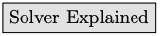button to see why starting from q = 1 leads Solver astray.

The explanation on the sheet makes it clear that the initial or starting value can play a critical role when numerical methods are utilized. This profit maximization problem has a sufficiently complicated surface that a numerical algorithm, such as Solver, cannot easily distinguish between local and global optimal solutions. There is no simple fix. The lesson is that you have to know the optimization problem you are dealing with and be careful interpreting the answers provided by a numerical algorithm.

The explanation of Solver’s failure involves the minimum point of the profit function and this provides an opportunity to explain the two roots in the quadratic formula. A picture, in this case, really is worth a thousand words.

STEP Click the 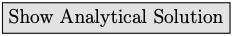button.

Cell Z17 has the other root from the quadratic formula (computed by adding instead of subtracting the square root term). Both roots are places where the profit function is flat (in the top right graph on the sheet). Notice how the dashed lines from the max and min profit points lead to points where marginal profit (\(m \pi\)) is zero. These are the two roots in the quadratic formula.

The two roots can also be seen in the canonical, bottom left graph as the two points where MR and MC intersect. Of course, we only care about the root that maximizes profits. One way to ensure that \(MR=MC\) yields a profit max is to make sure that \(MC < MR\) to the left of the intersection. In other words, MC cuts MR from below.

Numerical Methods to Derive the Supply Curve

STEP Set cell B8 back to 10 and P = 4 so Solver will converge to the local max at \(q = -15\).

STEP Run the Comparative Statics Wizard from \(P = 4\) with 0.05 sized shocks 100 times. Track the C4 and C8 cells as endogenous variables. You can safely ignore the warningyou are using the CSWiz to keep track of these cells, but will not include them as changing cells in the Solver dialog box.

Your results will look like those in the CS1 sheet. Notice that at low prices, the firm is producing nothing. This is the part of the supply curve where the firm shuts down to maximize profits.

The supply curve and inverse supply curves can be graphed with the CSWiz data, as shown in Figure 12.7 and the CS1 sheet. Of course, the tail runs along the quantity axis all the way to zero. Just as with the demand curve, \(q=f(P)\) is the supply curve and flipping the axes, \(P=f^{-1}(q)\), gives the inverse supply curve.

Figure 12.7: Deriving supply and inverse supply curves.

Source: DerivingSupply.xls!CS1.

Figure 12.7 applies our usual graphical exposition. The leftmost chart is the underlying graph from which the other charts are produced. We shock P and track \(q \mbox{*}\). This gives the supply curve.

Unlike the demand curve, however, notice that the supply curve follows MC as long as P is not below AVC. The discontinuity is at the minimum AVC. Row 32 of the CS1 sheet shows the break occurs for this cost function between $4.90 and $4.95. Prices below this minimum AVC value result in no quantity supplied since the firm shuts down.

Analytical methods can be used to find the discontinuity. First, we obtain an expression for AVC. \[\begin{gathered} %star suppresses line # TC=0.04q^3 - 0.9 q^2 + 10 q + 5\\ TVC=0.04q^3 - 0.9 q^2 + 10 q\\ AVC=\frac{TVC}{q}=0.04q^2 - 0.9 q + 10 \end{gathered}\] Then we take the derivative of AVC with respect to q and set it equal to zero to find its minimum point. \[\begin{gathered} %star suppresses line # \min\limits_{q} AVC=0.04q^2 - 0.9 q + 10\\ \frac{dAVC}{dq}=0.08q - 0.9 = 0\\ q \mbox{*} = \frac{0.9}{0.08}=11.25\end{gathered}\] By plugging this minimum value of output into the AVC function, we know the price at which the discontinuity kicks in. \[AVC[q=11.25]=0.04[11.25]^2 - 0.9 [11.25] + 10=4.9375\] In the CS1 sheet, the discontinuity occurs when price rises from $4.90 to $4.95. Our analytical work tells us that the discontinuity is exactly at $4.9375. Any price below this yields optimal q of zero.

Notice how we used the derivative to find the value of q at which the rate of change for the AVC curve was zero. This is the bottom of the U-shaped AVC curve and prices below this AVC result in shutting down. The lesson is that derivative is a tool that has a variety of uses.

The CS1 sheet also computes the price elasticity of supply in column E.

STEP Scroll down to see a comparison of slope and elasticities via the \(\Delta\) and derivative approaches.

In this case, the two approaches are not exactly the same because \(q \mbox{*}\) is non-linear in P. The sheet has all of the details in case you want to refresh your understanding of this concept.

Analytical Methods to Derive the Supply Curve

For the analytical approach, we use a different cost function to give us more practice. \[TC(q)=q^2+20\] With this quadratic cost function, we can set up and solve the PC firm’s profit maximization problem. Because it is a perfectly competitive firm, we know price is given and, thus, \(TR = Pq\). Therefore, the optimization problem is: \[\max\limits_{q} \pi=Pq-(q^2+20)\] We proceed by taking the derivative with respect to q and setting it to zero, then solving this first-order condition for optimal q. \[\frac{d \pi}{dq}=P-2q=0\] \[q \mbox{*}=\frac{1}{2}P\] This is the supply function. It gives the quantity supplied by a firm at every given price. For example, with \(P = 20\), \(q \mbox{*}\) = 10.

The inverse supply curve is found by expressing the equation as \(P=f(q)\). \[P=2q \mbox{*}\] The supply function tells us that \(q \mbox{*}\) increases by one-half fold for every increase in P. The size of the change in P does not matter since \(\frac{dq}{dP}\) is constant.

The price elasticity of supply is \(+1\). \[\begin{gathered} %star suppresses line # \frac{dq}{dP} = \frac{1}{2}\\ \frac{dq}{dP}\frac{q}{P} = \frac{1}{2}\frac{P}{\frac{1}{2}P}=1\end{gathered}\] We can compute the price elasticity of supply from one point to another. We know that at \(P=20\), \(q \mbox{*} = 10\). If \(P=30\), \(q \mbox{*} = 15\). A 50% rise in price led to a 50% increase in quantity supplied so the price elasticity of supply is \(+1\). The result is the same as the derivative approach because \(q \mbox{*}\) is linear in P.

A PC firm with a quadratic cost function will not shut down with any price greater than zero. By constructing its family of cost curves and graph of the optimal solution, we can see why. We begin with the cost curves. We know \(TVC = 2q\) and \(TFC = 20\). Then we can find the average and marginal curves. \[\begin{gathered} %star suppresses line # ATC(q)=\frac{TC}{q}=\frac{q^2+20}{q}=q+\frac{20}{q}\\ AVC(q)=\frac{TVC}{q}=\frac{q^2}{q}=q\\ MC(q)=\frac{dTC}{dq}=\frac{d(q^2+20)}{dq}=2q\end{gathered}\]

STEP Proceed to the Graphs sheet to see the four graph display of the optimal solution for this problem.

If \(P = 20\), then \(q \mbox{*} = 10\) and \(\pi \mbox{*} = \$80\). It is also obvious that there is no positive price at which this firm will shut down because AVC is simply a ray with slope \(+1\) out of the origin. Thus, price can never fall below AVC.

Notice also how there is only one point where \(MR=MC\), unlike the two intersections we saw with the cubic cost function. The quadratic cost function cannot produce the S-shape TC needed for the profit function to have a minimum profit at the bottom of a U-shape. The profit function in the top right graph has a single top of the hill (where \(m \pi = 0\)).

Points Off the Supply Curve

As we did with the demand curve (see Figure 4.12), we can explore the meaning of being off the supply curve. The interpretation is quite similar.

STEP Return to the CS1 sheet and manipulate the point off the supply and inverse supply curves with the scroll bar in column E.

Figure 12.8 shows what is on your screen, but in Excel you can move the red dot. As you do, the chosen q and profit for that quantity is displayed.

Figure 12.8: Points off the supply curve.

Source: DerivingSupply.xls!CS1.

Profits are maximized when you are on the supply curve. It is clear that the supply curve, like the demand curve, has a hidden third dimensionprofit for supply and utility for demand. The right most panel shows the mountain and how you approach the top at the optimal solution. The ridgeline connecting the mountain tops is the supply curve. Like the demand curve, points off the supply curve are associated with lower values of the objective function.

Notice how the point off the curve moves in a vertical fashion in the supply curve graph and horizontally on the inverse supply curve graph. This happens because price is constant (at P = 6.25). With the price on the x axis, points can be above or below the supply curve. Points off the inverse supply curve are to the right or left because P is on the y axis.

Finally, on the inverse supply curve, the inefficiency of being off the curve is obvious because output levels off the inverse supply curve means the firm is not choosing a point where \(MR (= P) = MC\).

The Supply Curve has Parents

Like demand and cost curves, supply is derived from an optimization problem. Knowing where key relationships come from separates introductory from more advanced economics and is an important aspect of mastering the economic way of thinking.

The supply curve is a comparative statics analysis of the effects on optimal quantity as price changes, ceteris paribus.

Unlike the demand curve, the supply curve has a discontinuity because the firm will shut down if price falls below AVC. The supply curve depends critically on the firm’s cost function. The inverse supply curve is simply MC above AVC and zero otherwise. The firm will choose that level of output where \(MR (=P) = MC\) as long as \(P > AVC\).

Like the demand curve, points off the supply curve are interpreted as inefficient solutions to the optimization problem. Although possible, no optimizing agent would choose a point off the supply (or demand) curve.

Exercises

1. What happens to the short run supply curve if wages rise? Explain. Use Word’s Drawing Tools to create a graph depicting your answer.
2. What happens to the inverse short run supply curve if wages rise? Explain. Use Word’s Drawing Tools to create a graph depicting your answer.
3. What happens to the short run supply curve if the rental rate of capital increases? Explain.
4. What happens to the short run supply curve if the price (P) increases? Explain.
5. Suppose a firm is off its short run supply curve, but at a point where \(MR = MC\). Use Word’s Drawing Tools to a draw the profit function for this situation and label a point Z that meets the supposed conditions.

References

The epigraph comes from page 92 of the 1897 English translation of Augustin Cournot’s Researches into the Mathematical Principles of the Theory of Wealth. This book was originally published in French in 1838. It is a remarkable worktruly far ahead of its time.

Cournot (pronounced coor–no) solves profit maximization problems for a variety of market structures, including monopoly, unlimited (today called perfect) competition, and intermediate cases of small numbers of firms. He uses derivatives and integrals with numerous supporting figures, including supply and demand with price on the x axis. Cournot was not bound by Marshall’s convention of P on the y axis since Marshall’s famous graphs of supply and demand would not appear until 1890.

The mathematical exposition was simply beyond the grasp of many readers in 1838 and the book languished in obscurity until the rise of mathematics in economics. You will hear Cournot’s name again in the chapter on Game Theory.