17.3: Tax Incidence and Deadweight Loss

Many goods and services are taxed. Sales taxes (also called value added or ad valorem taxes) are a percentage of the monetary amount spent; quantity taxes are levied per unit bought. Quantity taxes are applied, for example, to gasoline, alcohol, and cigarettes.

In chapter 3.4, we examined cigarette taxes. It was shown that, for a particular consumer, lump sum (fixed amount) taxes are better than quantity taxes. In this section, we turn from an analysis of taxes on the individual to their effect on society and the resource allocation problem.

We will use supply and demand in a partial equilibrium setting to evaluate the effects of taxes on goods and services allocated by the market. We work with quantity taxes because our linear supply and demand curves will shift vertically as the tax is applied. Sales taxes are harder to analyze, but the qualitative results we derive for quantity taxes carry over to sales taxes.

There are two basic issues:

1. Tax incidence: determining the tax split between buyer and seller.
2. Deadweight loss: evaluating the inefficiency generated by the tax.

Our work will show a counterintuitive proposition: It does not matter whether consumers or producers pay the tax. In the end, neither the tax burden nor the deadweight loss depends on who sends tax revenue to the government.

Our approach to the secondand more importantissue relies on comparing the output after the tax is imposed to the socially optimal output (based on maximizing consumers’ and producers’ surplus). Deviations from optimality are said to be inefficient solutions to society’s resource allocation problem. We will use deadweight loss to measure the inefficiency. This is known as welfare analysis, where welfare means the well-being of a person or group.

It Does Not Matter Who Sends the Tax Payment

Suppose you are renting an apartment for $700 a month. Suppose further that property taxes rise $100. If your landlord raises the rent to $800 a month and you agree, it is easy to see that you are paying for the entire tax increase. The landlord pays the property tax to the government, but you are bearing the burden of the tax.

But what if you refuse to pay the $100 increase and move out. The landlord cannot find anyone to rent the apartment for $800 and, eventually, agrees to rent the apartment for $725 a month to a new tenant. The computation of the tax burden is easy. The new tenant is bearing the burden of $25 or 25% of the tax increase, while the landlord’s burden is $75 or 75%.

No matter what the rent ends up being, the landlord sends the tax payment to the government, but that does not answer the question of who is really responsible for the tax. The landlord may be able to shift some of the tax onto the renter.

It turns out that the elasticities of demand and supply determine who bears the burden. The more inelastic, or price insensitive, the higher the burden.

Tax incidence is the analysis of who bears the burden of a tax. In a moment, we will be working with complicated supply and demand graphs, but the analysis is basically the same as the story of the tenant and the landlord.

Supplier Pays

For most products, the supplier or firm is responsible for collecting the tax when the good is purchased and for sending in the tax payments to the government. This is what is meant by “supplier pays.” Of course, we know that who collects and pays the tax is different from the tax incidence because anywhere from 0 to 100% of the tax may be shifted to the consumer.

The elasticities of supply and demand determine how the tax is split between consumer and firm.

STEP Open the Excel workbook Taxes.xls, read the Intro sheet, then go to the SupplierPays sheet.

The sheet has parameters for linear demand and supply curves. Initially, there is no tax so the equilibrium price is $100/unit and the equilibrium quantity is 125 units. Cell B17 shows that the government collects no revenue and cell E17 shows that there is no deadweight loss (because the market’s equilibrium quantity equals the socially optimal quantity).

The price elasticities at the initial equilibrium solution are \(\epsilon_D = - 0.4\) and \(\epsilon_S = 1.54\), for demand and supply. The sum of the absolute values is 1.94.

STEP Click on the scroll bar next to cell B14 five times to impose a tax.

A red line appears on the chart and it shifts with each click. Five clicks will set the tax at $50 and the spreadsheet will look like Figure 17.11.

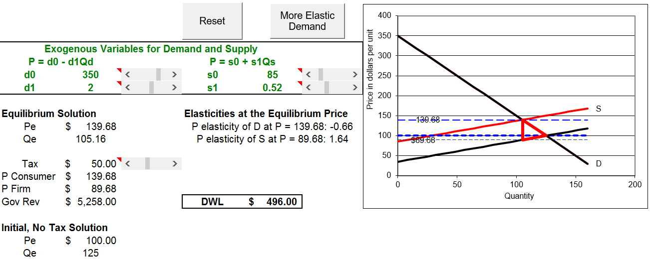
Figure 17.11: Supplier pays a $50 quantity tax.

Source: Taxes.xls!SupplierPays.

The inverse supply curve has shifted up by $50/unit because in order for the suppliers to offer a given quantity, they have to receive $50/unit more than the original supply curve (without the tax). They will not get to keep the extra $50 per unitthey have to send it to the government.

For example, to offer 125 units at the initial equilibrium solution, firms needed a price of $100, but now they will need $150/unit. The value of P is $150 for \(Q=125\) with the red line in Figure 17.11. Every quantity has the same $50 increase in price on the red line.

The spreadsheet displays the information we need to compute the tax incidence. We can see that the consumer is bearing the majority of the tax by looking at the new equilibrium price. The dashed line (and cell B15) shows the new \(P_e=139.68\). We can compute the fraction of the tax borne by the consumer: \(\frac{39.68}{50} \approx 79.4\%\). The supplier has managed to pass along all but about one-fifth of the tax to the consumer.

We can also use the absolute values of the pre-tax (initial) price elasticities to get the relative burdens for consumer and firm: \[1 - \frac{0.4}{1.94} \approx 79.4\% \text{ and } 1 - \frac{1.54}{1.94} \approx 20.6\%\] The Tax Incidence Formula to determine the share of the tax burden using demand and supply price elasticities is: \[1-\frac{\epsilon_i}{\epsilon_D+\epsilon_S} \text{ for } i=D, S\] The Tax Incidence Formula drops the minus sign for the price elasticity of demand and for the rest of this section, we will mean the absolute value when we refer to the price elasticity of demand.

The elasticity values from the spreadsheet and the Tax Incidence Formula make clear that the lower the price elasticity, the higher the tax incidence. As \(\epsilon_i \rightarrow 0\) (for either D or S), the burden (for D or S) goes to 100%. The consumer is paying four-fifths of tax in Figure 17.11 because demand is much more inelastic than supply at the initial equilibrium solution.

We will discuss tax incidence in more detail below, but we turn now to the second, more important issue, the welfare implications of per unit taxes.

With a $50 quantity tax, the SupplierPays sheet shows a deadweight loss of $496 in cell E17. The deadweight loss can be calculated by finding the difference of the maximum possible surplus minus the surpluses enjoyed by the consumers, producers, and government. This is equivalent to the (red) triangle on the chart, which is also known as a Harberger triangle.

We proceed carefully. Consumers’ surplus (CS) and producers’ surplus (PS) after the tax is imposed have both been reduced by the trapezoidal shapes in Figure 17.12. Clearly, CS has fallen by much more than PS. More importantly, however, is the fact that the deadweight loss (DWL) is not the sum of lost CS and PS because we have introduced a third playerthe government. They will get most of CS and PS lost in the form of tax revenue. The total tax payments of $5,280 is the area of the rectangle with height \(\$139.68 - \$89.68 = \$50\) and length 105.16 units of output.

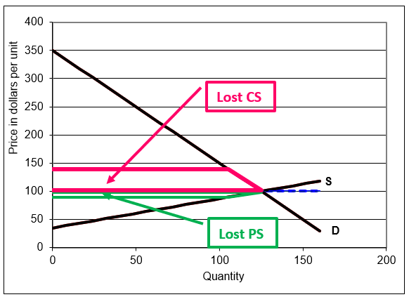
Figure 17.12: Lost CS and PS from the $50/unit tax.

Source: Taxes.xls!SupplierPays!AN.

Once we recognize that the tax has lowered CS and PS, but that part of the surplus is captured by the government, we can see that the deadweight loss is the Harberger (red) triangle in Figure 17.13, with area displayed in cell E17. The surplus in the Harberger triangle vaporizes into thin air, captured by no one.

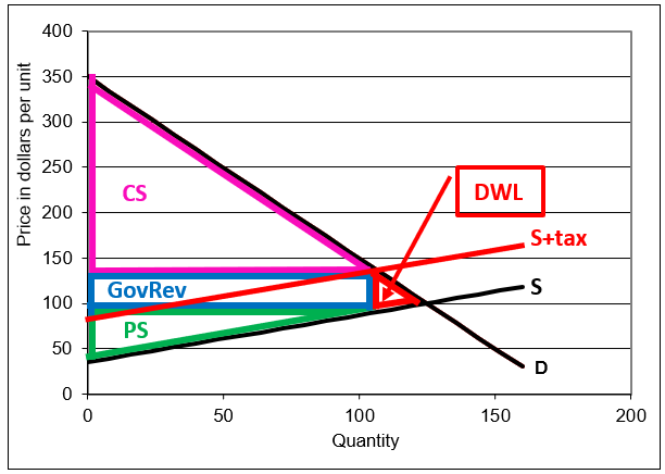
Figure 17.13: CS, PS, and GovRev from the $50/unit tax.

Source: Taxes.xls!SupplierPays!AN.

The height of the Harberger triangle is the price the consumer pays minus the price received by the firm, which is called the tax wedge. This distance is the amount of the tax. When you clicked five times to impose the tax, you could see the wedge expanding, creating a space between what the consumer pays and the firm receives.

The tax wedge takes surplus from consumers and producers, but this is not a problem. Presumably, the government is building schools, roads, and providing services. As long as someone gets the surplus, partial equilibrium surplus analysis counts it as a successful outcome.

Figure 17.13 shows, however, that the Harberger triangle goes to no one. This is a problem. Deadweight loss is surplus that simply vanishes. It is a loss of surplus that is not recouped by anyone.

The length of the DWL triangle is the distance from the new equilibrium quantity after the tax to the original equilibrium quantity. The bigger this distance, the greater is the distortion of the tax in terms of resource allocation.

STEP Click on cell E17 to see its formula. It simply computes the area of the red, Harberger triangle.

We summarize and repeat a few key ideas. Deadweight loss is a dollar measure of the distortion caused by the taxthe “market with a tax” scheme is no longer producing the optimal quantity. This is a misallocation of resources. Deadweight loss represents gains from trades that are not being exploited. There is $496 in value that no one is getting. It is simply vaporized and disappears into thin air.

The rectangle formed by the tax times the equilibrium quantity (after the tax is imposed) is a transfer from consumers and producers to the government. This does not count as deadweight loss because someone (the government) is getting it. The key to understanding deadweight loss is that it accrues to no oneit is unclaimed surplus and, therefore, pure waste.

Demander Pays

Suppose that instead of the firm it is the consumer who is responsible for collecting the quantity tax when the good is purchased and for sending in the tax payments to the government. This may seem a little strange at first, but there are cases where this occurs.

For example, if you buy online and the seller does not charge you state and local taxes, you are supposed to pay those taxes. At the dawn of the internet, this gave online retailers a big advantage over brick and mortar stores that included sales and other taxes in the total. Very few people pay taxes when they are not collected by the seller. Today, almost all online retailers include taxes.

For the purposes of comparing what happens when the buyer or seller pays the tax, forget about administrative costs or the fact that firms are much better tax collectors than consumers. We assume that consumers and firms will both comply and send the correct tax payment to the government even though that is obviously not true.

STEP Go to the DemanderPays sheet and impose a $50 tax. Pay attention to the screen as you click. You can watch the tax wedge emerge.

Figure 17.14 shows the result, with the DWL triangle displayed.

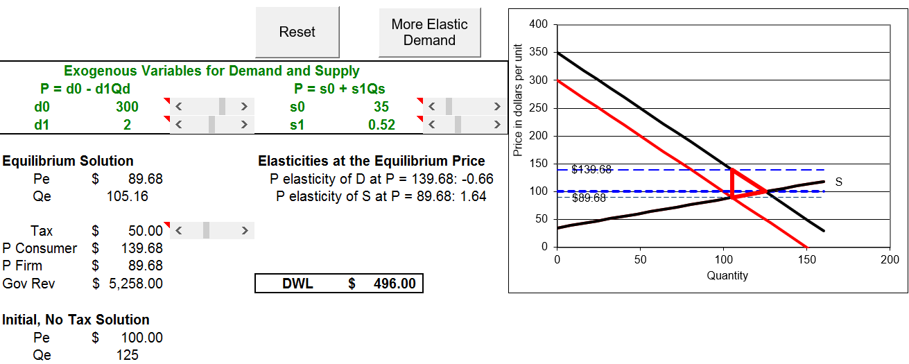
Figure 17.14: Demander pays a $50 quantity tax.

Source: Taxes.xls!DemanderPays.

This time, it is the demand curve that is shifting. Instead of the firm paying the tax, it is the consumer who must collect the tax and send in the payments. A $50 tax will shift the inverse demand curve down (not up) by $50 because each consumer is willing to buy any given quantity for $50 less than before since she will have to pay an additional $50 to the government for each unit purchased.

As before, a deadweight loss triangle appears when you impose the $50 tax. The tax drives a wedge between the total price the consumer pays and the amount the firm receives. This is the height of the triangle.

The deadweight loss triangle’s length is the difference between the initial and new \(Q_e\). The equilibrium quantity is driven down by the tax and, therefore, it no longer equals the socially optimal quantity. The tax causes an inefficient allocation of resources. The deadweight loss of $496 is a measure of the inefficiency caused by the tax.

The tax incidence can be found by computing the share of the tax paid by the consumer versus the firm. The sellers receive a price of $89.68 so they bear roughly $10 of the $50 tax. The consumer pays the firm $89.68 and the government $50 for each unit for a total price of $139.68. The buyer’s share of the tax is about 80%.

The government’s revenue is the $50 tax on each unit sold times the new equilibrium quantity, 105.16. This yields $5,258 and can be represented as a rectangle in the supply and demand graph.

It is obvious that these numbers are the same as the suppliers pays scenario, but a fun and memorable way to show that it does not matter who pays the government is to toggle back and forth between the two sheets.

STEP Click the SupplierPays sheet tab, then click the DemanderPays sheet tab. Repeat this several times while keeping your eye on the screen. What do you notice?

The chart is different, of course, and the d0 and s0 parameters are different because the demand and supply intercepts do change based on who collects the tax for the government. But the price paid by the consumer, the price received by the firm, government revenue, and, most importantly, equilibrium quantity and deadweight loss are all exactly the same.

There is no doubt about itthe tax incidence and deadweight loss do not depend at all on who physically collects and sends the tax payments to the government (compliance being equal). If it does not matter if the buyer or seller pays the tax, then what do tax incidence and deadweight loss depend on?

Elasticities Drive Tax Incidence and Deadweight Loss

The relative price elasticities of demand and supply determine both the tax incidence (the distribution of the tax burden) and the deadweight loss (the measure of inefficiency in the allocation of society’s resources).

The more inelastic is demand, given supply, the more the consumer will bear the burden of the tax and the lower the deadweight loss. The more inelastic is supply, given demand, the more the supplier bears the burden of the tax and the lower the deadweight loss.

We return to the apartment rent example to see how supply and demand analysis would work in an extreme case. If you agree to a $100 increase in rent, your demand for apartments is perfectly inelastic in this price range. The price increase from $700 to $800 has no effect on the quantity demanded. In this case, you bear the entire burden of the tax and there is no deadweight loss. The situation is depicted in Figure 17.15.

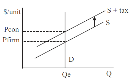Figure 17.15: Tax effects with perfectly inelastic demand.

If you, on the other hand, had to pay the property tax, you would be unable to shift it onto the landlord. In Figure 17.15, D would shift down, but it is a vertical line so it would shift on top of itself. The landlord would collect $700 from you (the initial equilibrium price) and you would pay an additional $100 to the government.

Our elasticity formula yields the same result. With perfectly inelastic demand, \(\epsilon_D = 0\). Thus, we have: \[1-\frac{\epsilon_D}{\epsilon_D+\epsilon_S} = 1 - \frac{0}{0+\epsilon_S} = 100\%\] This says the buyer bears the burden of the entire tax. Notice the formula does not have an input for who is writing the check to the governmentthat does not affect the outcome at all. The formula also tells us that \(\epsilon_S\) does not matter at all in the extreme case of perfectly inelastic demand.

The situation is reversed, of course, for the tax incidence if supply is perfectly inelastic. We would have a vertical S line that shifts up onto itself when the supplier pays the government. This leaves equilibrium price and quantity unchanged so the consumer pays the same amount as before and bears none of the tax burden. Once again, deadweight loss is zero.

Once again, the elasticity formula gives the same result. With \(\epsilon_S=0\), the \(\epsilon_D\) in the numerator and denominator cancel and the formula yields zero. This means the consumer bears no burden from a tax on a perfectly inelastically supplied good.

Of course, the main result that price elasticities determine tax incidence and deadweight loss applies in general and not just to these extreme cases. We can demonstrate this with the Excel workbook.

STEP To enable comparison, copy the SupplierPays sheet by right-clicking the sheet tab and selecting Move or Copy.) Select SupplierPays so the sheet is inserted before the SupplierPays sheet and check the Create a Copy box.

Excel inserts a new sheet in the workbook, named SupplierPays (2). We will apply the same $50 tax with a more elastic demand curve to see the effect on tax incidence and deadweight loss.

STEP Click the 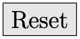button, then click the button in your new sheet.

A new, red inverse demand curve appears that is flatter, yet it goes through the initial equilibrium solution. The button simply sets the intercept and slope to 225 and 1, respectively. The price elasticity of demand at the initial equilibrium solution has risen (in absolute value) to \(- 0.8\) (as shown in cell E11).

It is important to not confuse slope and elasticity. The new, red inverse demand curve is more price elastic at \(P=100\) because it is flatter at that point. It is incorrect to say, however, that flatter lines are more elastic as a whole than steeper linesboth the initial and new inverse demand curves have varying elasticity all along the line. Thus, it does not make sense to say that flatter lines are more elastic. Elasticity refers to a percentage change response at a point. Only at \(P=100\) do we know that elasticity is higher for the flatter, red inverse demand curve.

STEP Click the tax scroll bar five times to impose a $50 per unit tax.

Figure 17.16 (and your screen) shows that the consumer bears less of the tax burden than before (but still more than the seller) and deadweight loss has risen.

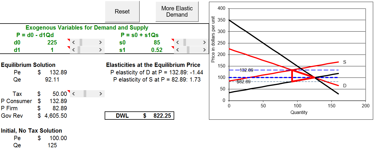
Figure 17.16: Tax effects with a more elastic D.

Source: Taxes.xls!SupplierPays.

With \(\epsilon_D = 0.8\) instead of 0.4, ceteris paribus, the tax incidence on the consumer has fallen because the price has risen only to $132.89 as opposed to $139.68 on the SupplierPays sheet. So, the consumer bears $32.89 of the $50 tax or \(\frac{32.89}{50} \approx 65.8\%\) of the tax. Notice that firms will now only net $82.89 per unit instead of $89.68 when \(\epsilon_D = 0.4\). Suppliers tax burden rises to 34.2%.

The tax incidence formula corroborates this result. \[1-\frac{\epsilon_D}{\epsilon_D+\epsilon_S} \text{ at } \epsilon_D=0.4 = 1 - \frac{0.4}{0.4 + 1.54} \approx 79.4\%\] \[1-\frac{\epsilon_D}{\epsilon_D+\epsilon_S} \text{ at } \epsilon_D=0.8 = 1 - \frac{0.8}{0.8 + 1.54} \approx 65.8\%\]

More importantly, deadweight loss has risen after the increase in the price of elasticity of demand from 0.4 to 0.8. Toggle back and forth from the original and new SupplierPays sheets to see that deadweight loss increases from $496 to $822.25.

While the height of the Harberger triangle has remained the same (the $50/unit tax), the length has increased because the new equilibrium quantity is farther from the initial \(Q_e=125\).

If you toggle back and forth a few times, you can see how the more elastic demand curve is creating a DWL triangle that is longer, but with the same $50 height. If you keep flattening the inverse demand curve (making sure that it passes through the initial equilibrium solution), the triangle keeps lengthening, but the height stays the same. A perfectly elastic (horizontal) D curve would produce the greatest deadweight loss possible.

STEP After thinking about it a bit, you can verify the claim above by using the control just to the right of the chart. Try all five scenarios.

With Equal Burden selected the demand and supply elasticities at \(P=100\) are the same so the $50 tax is split evenly. The consumer pays $125/unit and the firm receives $75/unit.

The bigger drop in equilibrium output with more elastic demand is also responsible for the fall in government revenues. Instead of collecting $5,258 in tax revenues, the government only gets $4,605.50. It gets $50/unit in both scenarios, but equilibrium quantity has fallen to 92.11 units with \(\epsilon_D=0.8\).

But neither the tax incidence nor the effect on government revenues is the highest priority issue. The top concern is the misallocation of society’s scarce resources caused by taxation. It is this that leads to a theory of optimal taxation.

Optimal Taxation

Figure 17.15 shows why it makes sense to tax inelastically demanded goods. If we could find perfectly inelastically demanded or supplied goods, we would tax them because then we would not distort the allocation of resources.

Our goal is to raise government revenue for needed projects by causing the smallest misallocation of resources. Thus, the optimal tax is the one that has the least deviation of equilibrium output from optimal output, which is equivalent to minimizing deadweight loss.

Clearly, it is better, ceteris paribus, to tax goods with low price elasticities of demand or supply. In the introduction to this section, gasoline, cigarettes, and alcohol were mentioned as goods that carry quantity taxes. It is no surprise that these goods are quite price inelastic at their usual sales prices.

Granted, there may be other reasons to tax these products (and we will see one of them in the section on externalities), but to the extent that government seeks revenue from taxing individual products, it should tax those that will not lead to large deadweight losses.

There is no quantity tax on Milky Ways, a scrumptious chocolate candy. Obviously, the government could never generate the same tax revenue from Milky Ways as gasoline, but even if it could, with so many substitutes, Milky Ways must be very price elastic. A tax on Milky Ways would lead to a great fall in equilibrium output. Government revenue would be quite low and deadweight loss very high.

Elasticity Rules

Public Finance (also known as Public Economics) is a subdiscipline of economics that includes the study of government tax policy. The theory of optimal taxation focuses on the best way to tax. The analysis in this section says that quantity taxes should not be applied to goods that are relatively price elastic because the deadweight loss will be high. Instead, by taxing goods with inelastic demand or supply curves, government can raise needed revenue with a minimum of distortion in the allocation of society’s resources.

This section also focused on the issue of tax incidence, who really bears the burden of a tax. This is a secondary issue compared to that of the optimal allocation of resources, but there is a surprising key result: It does not matter who collects the tax for the government (ignoring administrative costs and assuming equal compliance) because that party may be able to shift the tax onto someone else. Like deadweight loss, the tax incidence depends only on the elasticities of demand and supply. The more inelastic one of the curves is versus the other, the more that party will bear the burden of the tax. The Tax Incidence Formula sums this up conveniently: \[1-\frac{\epsilon_i}{\epsilon_D+\epsilon_S} \text{ for } i=D, S\]

The French economist Frederic Bastiat (1801 - 1850) had a clever way of explaining what economists do. In his final essay, titled "What is Seen and Unseen," Bastiat argues we need to be aware of invisible costs and effects.

Taxes are a good example. It is easy to think that property taxes are paid by property owners, but this is simply not necessarily true. What is seen, a tax payment, is not the whole story. It is amazing, but true, that who pays the tax bill is irrelevant. It is also amazing that price elasticities, which are unseen, completely determine tax incidence and deadweight loss.

Exercises

1. Do we get the same result if we have consumers or firms pay the tax to the government with a perfectly inelastic supply curve? To support your answer, use Word’s Drawing Tools to draw graphs. Explain the graphs and the result.
2. Use Word’s Drawing Tools to draw a graph where supply is more inelastic than demand at the initial equilibrium price. Apply a quantity tax. Comment on the tax incidence and deadweight loss.
3. In 1937, when Congress set up the Social Security system, it was decided that firms and workers each pay half of the total tax so the tax burden is equally shared. Today, workers and employers each pay 6.2% of wages up to maximum that changes each year. Do you think that by each party paying the same tax the burden is equally shared? Why or why not?
4. Suppose the demand for labor is more elastic than the supply of labor at the equilibrium wage. Use Use Word’s Drawing Tools to draw a graph that shows the tax incidence of the Social Security tax.

   Hint: You have to shift both demand and supply by the same amount, and then find the new equilibrium point.

References

The epigraph comes from page 168 of James R. Hines, Jr., “Three Sides of Harberger Triangles,” The Journal of Economic Perspectives, Vol. 13, No. 2 (Spring, 1999), pp. 167–188, www.jstor.org/stable/2647124. Hines explains that the theory of deadweight loss dates back to Dupuit, Jenkin, and Marshall, but Harberger’s papers in the 1950s and 1960s “illustrated the techniques, the usefulness, and the realistic possibility of performing such calculations, and in so doing, ushered in a new generation of applied normative work” (p. 168). For this reason, argues Hines, “Welfare loss triangles are ‘Harberger triangles’ because Harberger’s papers measured them, did so in a consistent manner, and assisted and encouraged a host of others to do likewise” (p. 185).

Arnold Harberger published a number of papers, but perhaps his key contribution was “The Measurement of Waste,” American Economic Review, Vol. 54, No. 3 (May, 1964), pp. 58–76, www.jstor.org/stable/1818490.