9: Perfect competition

9.1 The perfect competition paradigm

A competitive market is one that encompasses a very large number of suppliers, each producing a similar or identical product. Each supplier produces an output that forms a small part of the total market, and the sum of all of these individual outputs represents the production of that sector of the economy. Florists, barber shops, corner stores and dry cleaners all fit this description.

At the other extreme, a market that has just a single supplier is a monopolist. For example, the National Hockey League is the sole supplier of top-quality professional hockey games in North America; Hydro Quebec is a monopoly electricity distributor in Quebec; Via Rail is the only supplier of passenger rail services between Windsor, Ontario and the city of Quebec.

We use the word 'paradigm' in the title to this section: It implies that we will develop a model of supply behaviour for a market in which there are many small suppliers, producing essentially the same product, competing with one-another to meet the demands of consumers.

The structures that we call perfect competition and monopoly are extremes in the market place. Most sectors of the economy lie somewhere between these limiting cases. For example, the market for internet services usually contains several providers in any area – some provide using a fibre cable, others by satellite. The market for smart-phones in North America is dominated by two major players – Apple and Samsung (although there are several others). Hence, while these markets that have a limited number of suppliers are competitive in that they freely and perhaps fiercely compete for the buyer's expenditure, these are not perfectly competitive markets, because they do not have a very large number of suppliers.

In all of the models we develop in this chapter we will assume that the objective of firms is to maximize profit – the difference between revenues and costs.

The presence of so many sellers in perfect competition means that each firm recognizes its own small size in relation to the total market, and that its actions have no perceptible impact on the market price for the good or service being traded. Each firm is therefore a price taker—in contrast to a monopolist, who is a price setter.

The same 'smallness' characteristic was assumed when we examined the demands of individuals earlier. Each buyer takes the price as given. He or she is not big enough to be able to influence the price. In contrast, when international airlines purchase or lease aircraft from Boeing or Airbus, they negotiate over the price and other conditions of supply. The market models underlying these types of transactions are examined in Chapter 11.

Hence, when we describe a market as being perfectly competitive we do not mean that other market types are not competitive; all market structure are competitive in the sense that the suppliers wish to make profit, and they produce as efficiently as possible in order to meet that goal.

9.2 Market characteristics

The key attributes of a perfectly competitive market are the following:

1. There must be many firms, each one so small that it cannot influence price or quantity in the industry, and powerless relative to the entire industry.

2. The product must be standardized. Barber shops offer a standard product, but a Lexus differs from a Ford. Barbers tend to be price takers, but Lexus does not charge the same price as Ford, and is a price setter.

3. Buyers are assumed to have full information about the product and its pricing. For example, buyers know that the products of different suppliers really are the same in quality.

4. There are many buyers.

5. There is free entry and exit of firms.

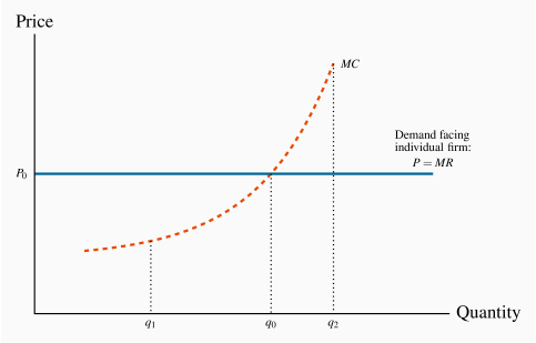
In terms of the demand curve that suppliers face, these market characteristics imply that the demand curve facing the perfectly competitive firm is horizontal, or infinitely elastic, as we defined in Chapter 4. In contrast, the demand curve facing the whole industry is downward sloping. The demand curve facing a firm is represented in Figure 9.1. It implies that the supplier can sell any output he chooses at the going price . He is a small player in the market, and variations in his output have no perceptible impact in the marketplace. But what quantity should he choose, or what quantity will maximize his profit? The profit-maximizing choice is his target, and the MC curve plays a key role in this decision.

9.3 The firm's supply decision

The concept of marginal revenue is key to analyzing the supply decision of an individual firm. We have used marginal analysis at several points to date. In consumer theory, we saw how consumers balance the utility per dollar at the margin in allocating their budget. Marginal revenue is the additional revenue accruing to the firm from the sale of one more unit of output.

In perfect competition, a firm's marginal revenue (MR) is the price of the good. Since the price is constant for the individual supplier, each additional unit sold at the price P brings in the same additional revenue. Therefore, P=MR. For example, whether a dry cleaning business launders 10 shirts or 100 shirts per day, the price charged to customers is the same. This equality holds in no other market structure, as we shall see in the following chapters.

Supply in the short run

Recall how we defined the short run in the previous chapter: Each firm's plant size is fixed in the short run, so too is the number of firms in an industry. In the long run, each individual firm can change its scale of operation, and at the same time new firms can enter or existing firms can leave the industry.

Perfectly competitive suppliers face the choice of how much to produce at the going market price: That is, the amount that will maximize their profit. We abstract for the moment on how the price in the marketplace is determined. We shall see later in this chapter that it emerges as the value corresponding to the intersection of the supply and demand curves for the whole market – as described in Chapter 3.

The firm's MC curve is critical in defining the optimal amount to supply at any price. In Figure 9.1, MC is the firm's marginal cost curve in the short run. At the price the optimal amount to supply is , the amount determined by the intersection of the MC and the demand. To see why, imagine that the producer chose to supply the quantity . Such an output would leave the opportunity for further profit untapped. By producing one additional unit beyond , the supplier would get in additional revenue and incur an additional cost that is less than in producing this unit. In fact, on every unit between and he can make a profit, because the MR exceeds the associated cost, MC. By the same argument, it makes no sense to increase output beyond , to for example, because the cost of such additional units of output, MC, exceeds the revenue from them. The MC therefore defines an optimal supply response.

Figure 9.1 The competitive firm's optimal output

Here, q₀ represents the optimal supply decision when the price is P₀. At output q₁ the cost of additional units is less than the revenue from such units and therefore it is profitable to increase output beyond q₁. Conversely, at q₂ the MC of production exceeds the revenue obtained, and so output should be reduced.

Application Box 9.1 The law of one price

If information does not flow then prices in different parts of a market may differ and potential entrants may not know to enter a profitable market.

Consider the fishermen off the coast of Kerala, India in the late 1990s. Their market was studied by Robert Jensen, a development economist. Prior to 1997, fishermen tended to bring their fish to their home market or port. This was cheaper than venturing to other ports, particularly if there was no certainty regarding price. This practice resulted in prices that were high in some local markets and low in others – depending upon the daily catch. Frequently fish was thrown away in low-price markets even though it might have found a favourable price in another village's fish market.

This all changed with the advent of cell phones. Rather than head automatically to their home port, fishermen began to phone several different markets in the hope of finding a good price for their efforts. They began to form agreements with buyers before even bringing their catch to port. Economist Jensen observed a major decline in price variation between the markets that he surveyed. In effect the 'law of one price' came into being for sardines as a result of the introduction of cheap technology and the relatively free flow of information.

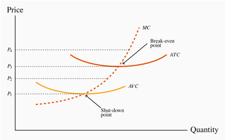
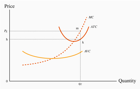
While the choice of the output is the best choice for the producer, Figure 9.1 does not tell us anything about profit. For that we need more information on costs. Accordingly, in Figure 9.2 the firm's AVC and ATC curves have been added to Figure 9.1. As explained in the previous chapter, the ATC curve includes both fixed and variable cost components, and the MC curve cuts the AVC and the ATC at their minima.

Figure 9.2 Short-run supply for the competitive firm

A price below P₁ does not cover variable costs, so the firm should shut down. Between prices P₁ and P₃, the producer can cover variable, but not total, costs and therefore should produce in the short run if fixed costs are 'sunk'. In the long run the firm must close if the price does not reach P₃. Profits are made if the price exceeds P₃. The short-run supply curve is the quantity supplied at each price. It is therefore the MC curve above P₁.

First, note that any price below , which corresponds to the minimum of the ATC curve, yields no profit, since it does not enable the producer to cover all of his costs. This price is therefore called the break-even price. Second, any price below , which corresponds to the minimum of the AVC, does not even enable the producer to cover variable costs. What about a price such as , that lies between these? The answer is that, if the supplier has already incurred some fixed costs, he should continue to produce, provided he can cover his variable cost. But in the long run he must cover all of his costs, fixed and variable. Therefore, if the price falls below , he should shut down, even in the short run. This price is therefore called the shut-down price. If a price at least equal to cannot be sustained in the long run, he should leave the industry. But at a price such as he can cover variable costs and therefore should continue to produce in the short run. His optimal output at is defined by the intersection of the line with the MC curve. The firm's short-run supply curve is, therefore, that portion of the MC curve above the minimum of the AVC.

To illustrate this more concretely, consider again the example of our snowboard producer, and imagine that he is producing in a perfectly competitive marketplace. How should he behave in response to different prices? Table 9.1 reproduces the data from Table 8.2.

Table 9.1 Profit maximization in the short run

Labour	Output	Total	Average	Average	Marginal	Total	Profit
		Revenue $	Variable	Total Cost	Cost $	Cost $
			Cost	$
L	Q	TR	AVC	ATC	MC	TC	TR-TC
0	0					3,000
1	15	1,050	66.67	266.67	66.67	4,000	–2,950
2	40	2,800	50.0	125.0	40.0	5,000	–2,200
3	70	4,900	42.86	85.71	33.33	6,000	–1,100
4	110	7,700	36.36	63.64	25.0	7,000	700
5	145	10,150	34.48	55.17	28.57	8,000	2,150
6	175	12,250	34.29	51.43	33.33	9,000	3,250
7	200	14,000	35.0	50.0	40.0	10,000	4,000
8	220	15,400	36.36	50.0	50.0	11,000	4,400
9	235	16,450	38.30	51.06	66.67	12,000	4,450
10	240	16,800	41.67	54.17	200.0	13,000	3,800

Output Price=$70; Wage=$1,000; Fixed Cost=$3,000. The shut-down point occurs at a price of , where the AVC attains a minimum. Hence no production, even in the short run, takes place unless the price exceeds this value. The break-even level of output occurs at a price of , where the ATC attains a minimum.

The shut-down price corresponds to the minimum value of the AVC curve.

The break-even price corresponds to the minimum of the ATC curve.

The firm's short-run supply curve is that portion of the MC curve above the minimum of the AVC.

Suppose that the price is $70. How many boards should he produce? The answer is defined by the behaviour of the MC curve. For any output less than or equal to 235, the MC is less than the price. For example, at L=9 and Q=235, the MC is $66.67. At this output level, he makes a profit on the marginal unit produced, because the MC is less than the revenue he gets ($70) from selling it.

But, at outputs above this, he registers a loss on the marginal units because the MC exceeds the revenue. For example, at L=10 and Q=240, the MC is $200. Clearly, 235 snowboards is the optimum. To produce more would generate a loss on each additional unit, because the additional cost would exceed the additional revenue. Furthermore, to produce fewer snowboards would mean not availing of the potential for profit on additional boards.

His profit is based on the difference between revenue per unit and cost per unit at this output: (P–ATC). Since the ATC for the 235 units produced by the nine workers is $51.06, his profit margin is per board, and total profit is therefore .

Let us establish two other key outputs and prices for the producer. First, the shut-down point is the minimum of his AVC curve. Table 9.1 indicates that the price must be at least $34.29 for him to be willing to supply any output, since that is the value of the AVC at its minimum. Second, the minimum of his ATC is at $50. Accordingly, provided the price exceeds $50, he will cover both variable and fixed costs and make a maximum profit when he chooses an output where P=MC, above . It follows that the short-run supply curve for Black Diamond Snowboards is the segment of the MC curve in Figure 8.4 above the AVC curve.

Given that we have developed the individual firm's supply curve, the next task is to develop the industry supply curve.

Industry supply in the short run

In Chapter 3 it was demonstrated that individual demands can be aggregated into an industry demand by summing them horizontally. The industry supply is obtained in exactly the same manner—by summing the firms' supply quantities across all firms in the industry.

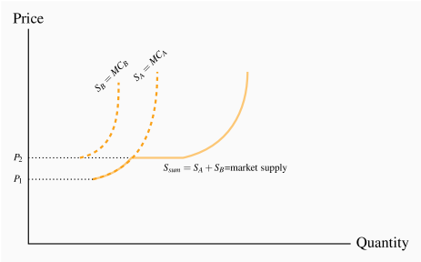
To illustrate, imagine we have many firms, possibly operating at different scales of output and therefore having different short-run MC curves. The MC curves of two of these firms are illustrated in Figure 9.3. The MC of A is below the MC of B; therefore, B likely has a smaller scale of plant than A. Consider first the supply decisions in the price range P₁ to P₂. At any price between these limits, only firm A will supply output – firm B does not cover its AVC in this price range. Therefore, the joint contribution to industry supply of firms A and B is given by the MC curve of firm A. But once a price of P₂ is attained, firm B is now willing to supply. The schedule is the horizontal addition of their supply quantities. Adding the supplies of every firm in the industry in this way yields the industry supply.

Industry supply (short run) in perfect competition is the horizontal sum of all firms' supply curves.

Figure 9.3 Deriving industry supply

The marginal cost curves for firms A and B indicate that at any price below P₁ production is unprofitable and supply is therefore zero for both firms. At prices between P₁ and P₂ firm A is willing to supply, but not firm B. Consequently the market supply comes only from A. At prices above P₂ both firms are willing to supply. Therefore the market supply is the horizontal sum of each firm's supply.

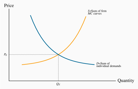
Industry equilibrium

Consider next the industry equilibrium. Since the industry supply is the sum of the individual supplies, and the industry demand curve is the sum of individual demands, an equilibrium price and quantity (P_E,Q_E) are defined by the intersection of these industry-level curves, as in Figure 9.4. Here, each firm takes P_E as given (it is so small that it cannot influence the going price), and supplies an amount determined by the intersection of this price with its MC curve. The sum of such quantities is therefore Q_E.

Short-run equilibrium in perfect competition occurs when each firm maximizes profit by producing a quantity where P=MC, provided the price exceeds the minimum of the average variable cost.

Figure 9.4 Market equilibrium

The market supply curve S is the sum of each firm's supply or MC curve above the shut-down price. D is the sum of individual demands. The market equilibrium price and quantity are defined by P_E and Q_E.

9.4 Dynamics: Entry and exit

We have now described the market and firm-level equilibrium in the short run. However, this equilibrium may be only temporary; whether it can be sustained or not depends upon whether profits (or losses) are being incurred, or whether all participant firms are making what are termed normal profits. Such profits are considered an essential part of a firm's operation. They reflect the opportunity cost of the resources used in production. Firms do not operate if they cannot make a minimal, or normal, profit level. Above such profits are economic profits (also called supernormal profits), and these are what entice entry into the industry.

Recall from Chapter 7 that accounting and economic profits are different. The economist includes opportunity costs in determining profit, whereas the accountant considers actual revenues and costs. In the example developed in Section 7.2 the entrepreneur recorded accounting profit, but not economic profit. Suppose now that the numbers were slightly different, and are as defined in Table 9.2: Felicity invests $250,000 in her business in the form of capital, as before. But she now has gross revenues of $165,000 and incurs a cost of $90,000 to buy the clothing wholesale that she then sells retail. She pays herself a salary of $35,000. If these numbers represent her balance sheet, then she records an accounting profit of $40,000.

Her economic profit calculation must include opportunity costs. The opportunity cost of tying up $250,000 of capital, if the interest rate is 4%, amounts to $10,000. In addition, if Felicity could earn $55,000 in her best alternative job then an additional implicit cost of $20,000 must be considered. When these two opportunity (or implicit) costs are added to the balance sheet, her profit is reduced to $10,000. This is her economic profit. If Felicity's economic profit is representative of the retail clothing sector of the economy, then that profitability should attract new entrepreneurs. Our conclusion is that this sector of the economy should experience new entrants and hence an outward shift of the supply curve. In contrast, in the numerical example considered in Section 7.2, Felicity was experiencing losses (negative economic profits), and in the longer term she would have to consider leaving the business. If she and other suppliers exited, then the market supply curve would shift back to the left – representing a reduction in supply.

The critical point in this distinction between accounting and economic cost is that the decision to enter or leave a market in the longer term is based on what the entrepreneur can earn in the wider market place. That is, economic profits rather than accounting profits will determine the equilibrium number of firms in the long term. In terms of our cost curves, we will assume that the full economic costs are included in the various curves that we use. Consequently any profits (or losses) that arise are based upon the full economic costs of the firm's operation.

Let us return to our graphical analysis, and begin by supposing that the market equilibrium described in Figure 9.4 results in profits being made by some firms. Such an outcome is described in Figure 9.5, where the price exceeds the ATC. At the price , a profit-making firm supplies the quantity , as determined by its MC curve. On average, the cost of producing each unit of output, , is defined by the point on the ATC at that output level, point k. Profit per unit is thus given by the value (m–k) – the difference between revenue per unit and cost per unit. Total (economic) profit is therefore the area , which is quantity times profit per unit.

Figure 9.5 Short-run profits for the firm

At the price P_E, determined by the intersection of market demand and market supply, an individual firm produces the amount Q_E. The ATC of this output is k and therefore profit per unit is mk. Total profit is therefore P_Emkhmk=TR–TC.

Figure 9.6 Entry of firms due to economic profits

If economic profits result from the price P_E new firms enter the industry. This entry increases the market supply to and the equilibrium price falls to . Entry continues as long as economic profits are present. Eventually the price is driven to a level where only normal profits are made, and entry ceases.

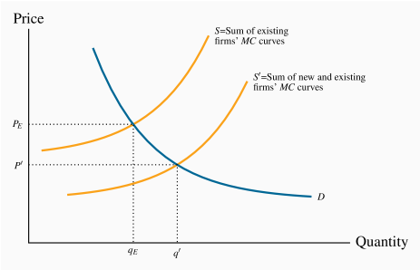
While represents an equilibrium for the firm, it is only a short-run, or temporary, equilibrium for the industry. The assumption of free entry and exit implies that the presence of economic profits will induce new entrepreneurs to enter and start producing. The impact of this dynamic is illustrated in Figure 9.6. An increased number of firms shifts supply rightwards to become , thereby increasing the amount supplied at any price. The impact on price of this supply shift is evident: With an unchanged demand, the equilibrium price must fall.

How far will the price fall, and how many new firms will enter this profitable industry? As long as economic profits exist new firms will enter and the resulting increase in supply will continue to drive the price downwards. But, once the price has been driven down to the minimum of the ATC of a representative firm, there is no longer an incentive for new entrepreneurs to enter. Therefore, the long-run industry equilibrium is where the market price equals the minimum point of a firm's ATC curve. This generates normal profits, and there is no incentive for firms to enter or exit.

In developing this dynamic, we began with a situation in which economic profits were present. However, we could have equally started from a position of losses. With a market price between the minimum of the AVC and the minimum of the ATC in Figure 9.5, revenues per unit would exceed variable costs but not total costs per unit. When firms cannot cover their ATC in the long run, they will cease production. Such closures must reduce aggregate supply; consequently the market supply curve contracts, rather than expands as it did in Figure 9.6. The reduced supply drives up the price of the good. This process continues as long as firms are making losses. A final industry equilibrium is attained only when the price reaches a level where firms can make a normal profit. Again, this will be at the minimum of the typical firm's ATC.

Accordingly, the long-run equilibrium is the same, regardless of whether we begin from a position in which firms are incurring losses, or where they are making profits.

9.5 Long-run industry supply

When aggregating the firm-level supply curves, as illustrated in Figure 9.3, we did not assume that all firms were identical. In that example, firm A has a cost structure with a lower AVC curve, since its supply curve starts at a lower dollar value. This indicates that firm A may have a larger plant size than firm B – one that puts A closer to the minimum efficient scale region of its long-run ATC curve.

Figure 9.7 Firms with different plant sizes

Firm B cannot compete with Firm A in the long run given that B has a less efficient plant size than firm A. The equilibrium long-run price equals the minimum of the LAC. At this price firm B must move to a more efficient plant size or make losses.

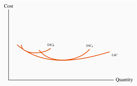
Can firm B survive with his current scale of operation in the long run? Our industry dynamics indicate that it cannot. The reason is that, provided some firms are making economic profits, new entrepreneurs will enter the industry and drive the price down to the minimum of the ATC curve of those firms who are operating with the lowest cost plant size. B-type firms will therefore be forced either to leave the industry or to adjust to the least-cost plant size—corresponding to the lowest point on its long-run ATC curve. Remember that the same technology is available to all firms; they each have the same long-run ATC curve, and may choose different scales of operation in the short run, as illustrated in Figure 9.7. But in the long run they must all produce using the minimum-cost plant size, or else they will be driven from the market.

This behaviour enables us to define a long-run industry supply. The long run involves the entry and exit of firms, and leads to a price corresponding to the minimum of the long-run ATC curve. Therefore, if the long-run equilibrium price corresponds to this minimum, the long-run supply curve of the industry is defined by a particular price value—it is horizontal at the price corresponding to the minimum of the LATC. More or less output is produced as a result of firms entering or leaving the industry, with those present always producing at the same unit cost in a long-run equilibrium.

Figure 9.8 Long-run dynamics

The LR equilibrium price P_E is disturbed by a shift in demand from D₁ to D₂. With a fixed number of firms, P₂ results. Profits accrue at this price and entry occurs. Therefore the SR supply shifts outwards until these profits are eroded and the new equilibrium output is Q₂. If, instead, D falls to D₃ then firms exit because they make losses, S shifts back until the price is driven up sufficiently to restore normal profits. Different outputs are supplied in the long run at the same price P_E, therefore the long-run supply is horizontal at P_E.

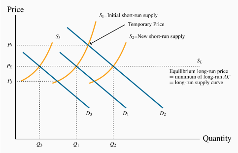
This industry's long-run supply curve, S_L, and a particular short-run supply are illustrated in Figure 9.8. Different points on S_L are attained when demand shifts. Suppose that, from an initial equilibrium Q₁, defined by the intersection of D₁ and S₁, demand increases from D₁ to D₂ because of a growth in income. With a fixed number of firms, the additional demand can be met only at a higher price (P₂), where each existing firm produces more using their existing plant size. The economic profits that result induce new operators to produce. This addition to the industry's production capacity shifts the short-run supply outwards and price declines until normal profits are once again being made. The new long-run equilibrium is at Q₂, with more firms each producing at the minimum of their long-run ATC curve, P_E.

The same dynamic would describe the industry reaction to a decline in demand—price would fall, some firms would exit, and the resulting contraction in supply would force the price back up to the long-run equilibrium level. This is illustrated by a decline in demand from D₁ to D₃.

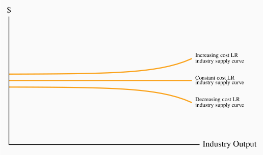
Increasing and decreasing cost industries

While a horizontal long-run supply is the norm for perfect competition, in some industries costs increase with the scale of industry output; in others they decrease. This may be because all of the producers use a particular input that itself becomes more or less costly, depending upon the amount supplied.

Figure 9.9 Increasing and decreasing cost industries

When individual-supplier costs rise as the output of the industry increases we have an increasing cost supply curve for the industry in the long run. Conversely, when the costs of individual suppliers fall with the scale of the industry, we have a decreasing cost industry.

Decreasing cost sectors are those that benefit from a decline in the prices of their inputs as the size of their market expands. This is frequently because the suppliers of the inputs themselves can benefit from scale economies as a result of expansion in the market for the final good. A case in point has been the computer market, or the tablet market: As output in these markets has grown, the producers of videocards and random-access memory have benefited from scale economies and thus been able to sell these components at a lower price to the manufacturers of the final goods. An example of an increasing cost market is the market for landings and take-offs at airports. Airports are frequently limited in their ability to expand their size and build additional runways. In such markets, as use grows, planes about to land may have to adopt a circling holding pattern, while those departing encounter clearance delays. Such delays increase the time costs to passengers and the fuel and labour costs to the suppliers. Decreasing and increasing industry costs are reflected in the long-run industry supply curve by a downward-sloping segment or an upward sloping segment, as illustrated in Figure 9.9.

Increasing (decreasing) cost industry is one where costs rise (fall) for each firm because of the scale of industry operation.

9.6 Globalization and technological change

Globalization and technological change have had a profound impact on the way goods and services are produced and brought to market in the modern world. The cost structure of many firms has been reduced by outsourcing to lower-wage economies. Furthermore, the advent of the communications revolution has effectively increased the minimum efficient scale for many industries, as illustrated in Chapter 8 (Figure 8.7). Larger firms are less difficult to manage nowadays, and the LAC curve may not slope upwards until very high output levels are attained. The consequence is that some industries may not have sufficient "production space" to sustain a large number of firms. In order to reap the advantages of scale economies, firms become so large that they can supply a significant part of the market. They are no longer so small as to have no impact on the price.

Outsourcing and easier communications have in many cases simply eliminated many industries in the developed world. Garment making is an example. Some decades ago Quebec was Canada's main garment maker: Brokers dealt with 'cottage-type' garment assemblers outside Montreal and Quebec City. But ultimately the availability of cheaper labour in the developing world combined with efficient communications undercut the local manufacture. Most of Canada's garments are now imported. Other North American and European industries have been impacted in similar ways. Displaced labour has had to reskill, retool, reeducate itself, and either seek alternative employment in the manufacturing sector, or move to the service sector of the economy, or retire.

Globalization has had a third impact on the domestic economy, in so far as it reduces the cost of components. Even industries that continue to operate within national boundaries see a reduction in their cost structure on account of globalization's impact on input costs. This is particularly in evidence in the computing industry, where components are produced in numerous low-wage economies, imported to North America and assembled into computers domestically. Such components are termed intermediate goods.

9.7 Efficient resource allocation

Economists have a particular liking for competitive markets. The reason is not, as is frequently thought, that we love competitive battles; it really concerns resource allocation in the economy at large. In Chapter 5 we explained why markets are frequently an excellent vehicle for transporting the economy's resources to where they are most valued: A perfectly competitive marketplace in which there are no externalities results in resources being used up to the point where the demand and supply prices are equal. If demand is a measure of marginal benefit and supply is a measure of marginal cost, then a perfectly competitive market ensures that this condition will hold in equilibrium. Perfect competition, therefore, results in resources being used efficiently.

Our initial reaction to this perspective may be: If market equilibrium is such that the quantity supplied always equals the quantity demanded, is not every market efficient? The answer is no. As we shall see in the next chapter on monopoly, the monopolist's supply decision does not reflect the marginal cost of resources used in production, and therefore does not result in an efficient allocation in the economy.

Key Terms

Exercises for Chapter 9