The short run in macroeconomics is defined by assuming a specific set of conditions in the economy. These are:
- There are constant prices for factors of production, especially money wage rates for labour.
- The supply of labour, the stock of capital, and the state of technology are fixed.
Short run: a time frame in which factor prices, supplies of factors of production, and technology are fixed by assumption.
In the short run, changes in output involve changes in the employment of labour and in the use of plant and equipment, but these changes are not sustainable over longer time periods. Furthermore, because supplies of factor inputs and technology are fixed, there is no sustained growth in real GDP. We leave that topic for a later chapter.
The national accounts we studied in Chapter 4 describe and measure economic activity in terms of an accounting framework used to measure aggregate expenditures, outputs, and incomes. But the accounting framework simply measures what has happened in the recent past. It does not explain the level of economic activity and prices or the reasons for changes in output and prices from time to time.
For that we need an analytical framework that looks at cause and effect. An aggregate demand (AD) and aggregate supply (AS) model is such an analytical framework. It helps us understand the conditions that determine output and prices, and changes in output and prices over time.
AD/AS model: a framework used to explain the behaviour of real output and prices in the national economy.
The short-run AD/AS model builds on the national accounts framework. Aggregate demand is the relationship between aggregate expenditure on final goods and services and the general price level. Real GDP by the expenditure approach measures this expenditure at the price level given by the GDP deflator. Aggregate supply is the relationship between the output of goods and services produced by business and the general price level. Real GDP by the income approach measures this output, and the corresponding real incomes. The price level is again the GDP deflator. National accounts tell us that, by definition, these measured outputs and incomes are equal. AD and AS functions describe expenditure plans, outputs, and prices using the national accounts framework. This distinction between measured and planned expenditure and output is important. Planned expenditure is the current output households and businesses would want to buy at different levels of income and price. Output is what businesses actually produce. Planned expenditure and the actual output produced by business may not be the same.
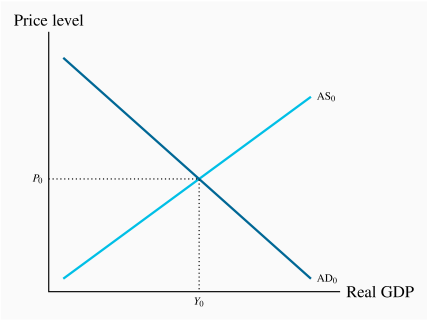
Figure 5.1 gives us a first look at output, real income, and prices for a specific year using an aggregate demand and aggregate supply diagram. The price level as measured by the GDP deflator is measured on the vertical axis. Real output and income are measured on the horizontal axis. The point of intersection of the AD and AS lines shows that real output by the expenditure approach, Y0, is equal to real income by the income approach at the price level P0, as required by national accounts. It also shows planned aggregate expenditures equal to the current output of goods and services. However, we need to explain the aggregate demand and aggregate supply relationships indicated by the slopes and positions of the AD and AS lines in the diagram before we use the model to study output and prices.
Equilibrium GDP: AD=AS, planned expenditure equals current output and provides business revenues that cover current costs including expected profit.
Aggregate demand (AD) is planned aggregate expenditure on final goods and services at different price levels when all other conditions are constant. This relationship is examined in detail in the chapters that follow. A downward sloping AD curve means the relationship between planned aggregate expenditure and the general price level is negative. A higher price level reduces the expenditures planned by households, businesses, and residents of other countries. Lower price levels increase those expenditure plans.
Aggregate demand: planned aggregate expenditure on final goods and services at different price levels, all other conditions remaining constant.
Aggregate Supply (AS) is the output of final goods and services business produces at different price levels when other conditions are constant. The upward sloping AS curve in Figure 5.1 assumes that the relationship between the quantity of goods and services produced and the price level is positive. Prices and output rise or fall together. We will examine this relationship in more detail below and in later chapters.
As we can see in the diagram, changes in either AD or AS would result in changes in the point of intersection of AD and AS and in equilibrium P and Y. But the important question is: What economic conditions and events determine the positions and slopes of AD and AS? The model is a tool for economic analysis that will only be useful when we know how it works and how to operate it.
Aggregate supply: the output of final goods and services businesses would produce at different price levels, all other conditions held constant.
Aggregate demand
Aggregate Demand and the market demand for an individual product are different. In our discussion of the market for an individual product in Chapter 3, demand is based on the assumptions that incomes and prices of other products are constant. Then a rise in the price of the product makes the product more expensive relative to income and relative to other products. As a result, people buy less of the product. Alternatively, if price falls people buy more.
The link between the general price level and aggregate demand is different. We cannot assume constant incomes and prices of other products. In the aggregate economy a rise in the price level raises money incomes by an equal amount. A 10 percent rise in the general price level is also a 10 percent rise in money incomes. Changes in the price level do not make goods and services either more or less affordable, in terms of incomes. There is no direct price incentive to change aggregate expenditure.
Furthermore, if prices of individual goods and services do not rise or fall in the same proportion as the general price level, the distribution of aggregate expenditure among goods and services may change without a change in aggregate expenditure. If, for example, the general price level is pushed up because oil and commodity prices rise, and expenditure on those products rises in the short run because there are no alternatives, expenditures on other goods and services fall. Aggregate expenditure is unchanged.
As a result, we cannot explain the negative relationship between the general price level and aggregate expenditure as we would explain demand for an individual good or service. Nor can we simply add up all the demands for individual products and services to get aggregate demand. The assumptions of constant incomes and other product prices that underlie market demand do not hold in the aggregate. Different explanations are needed.
Money and financial markets play key roles in the explanation of the price-quantity relationship in aggregate demand and the negative slope of AD as follows:
- Changes in the price level (P) change demand and supply conditions in financial markets. Higher prices raise interest rates and lower prices lower interest rates.
- Interest rates determine costs of credit and foreign exchange rates. Higher interest rates reduce expenditures on goods and services, lower interest rates stimulate expenditure.
- The responsiveness of expenditures to changes in interest rates determines the extent of the change in expenditure (Y) as a result of a change in the price level (P).
- Changes in expenditure then feed back to offset some of the change in financial conditions.
Chapters 8, 9 and 10 examine these financial markets and their effects on expenditure.
The result is a negative relationship between the price level and aggregate expenditure and a negatively sloped AD curve.
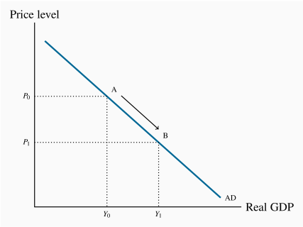
In Figure 5.2, the negatively sloped AD line shows planned aggregate expenditures at different price levels, on the assumption that the money supply and anything other than price that might affect expenditure plans are held constant. If the price level falls from P0 to P1, the movement along AD from A to B shows the negative relationship between planned aggregate expenditure and price. A rise in price would reduce planned expenditure as shown by moving up the AD curve.
The position of the AD curve depends on all the conditions other than price that affect aggregate expenditure plans. We study these other conditions in detail in later Chapters 6 and 7.
Aggregate supply
Aggregate Supply (AS) is the output of final goods and services businesses would produce at different price levels. The aggregate supply curve is based on the following key assumptions:
- Prices of the factors of production—the money wage rate for labour in particular—are constant.
- The stock of capital equipment—the buildings and equipment used in the production process—and the technology of production are constant.
From national accounts we know that the costs of production include labour costs, business and investment incomes and depreciation. Market prices depend on those costs per unit of output and the output and price setting decisions by producers. Aggregate supply is usually described as a positive relationship between quantities of goods and services businesses are willing to produce and prices. Higher outputs of final goods and services and higher prices go together.
This relationship between aggregate output, costs and prices reflects two different market conditions on the supply side. In some markets, particularly those for commodities and standardized products, supply and demand in international markets establish price. Producers of those products are price takers. They decide how much labour and plant capacity to employ to produce based on market price.
Broadly speaking, in these industries cost per unit of output are increasing with increasing output. Employing more labour and plant capacity means expanding into less productive land and natural resource inputs. Mining gold or extracting bitumen from oil sands are good examples. A rise in price justifies expanding the output of higher cost mines and oil wells. However, many raw material markets are like this including those for agricultural products, forestry products, base metals and natural gas. When market price changes these producers respond by changing their outputs.
In other parts of the economy producers are price setters. Major manufacturing and service industries like auto producers, banks and wireless phone companies face market conditions that are different from those of commodity producers. They set prices based on costs of production and sales and profit targets, and supply the number of cars or bank services or cell phone accounts that are in demand at those prices.
In these industries costs per unit of output are constant over a wide range of current outputs. Money wage rates are fixed, the capacity to produce output is flexible and productivity is constant. If demand for their product or service increases they can supply more by hiring more employees at existing wage rates and selling more output at existing prices. Industries like major manufacturing, retail services, financial services, hospitality services, and professional services are some examples. Output and changes in output are determined by demand.
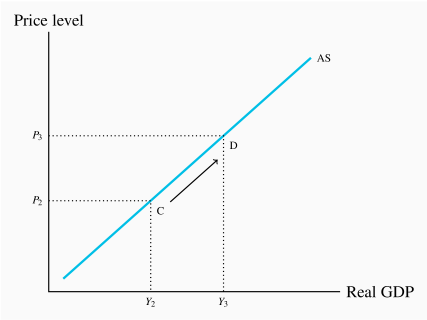
The upward-sloping aggregate supply curve in Figure 5.3 captures both market conditions to show the output producers are willing to produce and the price level. The aggregate supply curve is drawn based on the assumptions that money wage rates and all other conditions except price that might affect output decisions are constant. As we will see in later chapters, money wage rates and productivity are the most important of these conditions. They determine the position of the AS curve.
The slope of the AS curve depends on changes in cost per unit of output and price changes if aggregate output changes. As a result it reflects the structure of industry. In Canada, for example Table 4.2 shows that about 70 percent of real GDP comes from service producing industries. Consequently we would expect a smaller positive slope in the AS curve than in Figure 5.3.
In Figure 5.3, if price were P2 the AS curve shows that business would be willing to produce aggregate output Y2, which would generate an equal flow of real income. A rise in aggregate output from Y2 to Y3 would mean a rise in price to P3 to meet the increased costs and profits associated with output at this level. Changes in output or price, holding all other conditions constant, move the economy along the AS curve. Moving from point C to point D in the diagram shows this relationship.
On the other hand, a change in any of the conditions assumed to be constant will shift the entire AS curve. A rise in money wage rates, for example, would increase labour costs per unit of output (W/Y) at every level of output. The AS curve would shift up vertically as prices rose in order to cover the increased unit labour costs.

 and
and  planned expenditures on final goods and services are equal to real GDP at
  .
.


