10.4: Monetary Policy Rules

Most central banks now use interest rates as the main instrument of monetary policy. But how does a central bank decide what rate of interest to set and when to change its settings of the interest rate? What lies behind the announcement of the overnight rate by the Bank of Canada or the setting of the federal funds rate in the United States? How are these interest rate decisions related to economic variables? Professor John Taylor of Stanford University found that most central banks, in fact, adjust interest rates in response to changes in two variables, output and inflation.

This finding was contentious. It implied monetary supply targets no longer played a role in decisions about setting interest rates. Instead, the interest rate target was and is set based on expected inflation and expected output relative to the central bank's inflation target and the economy's potential output.

A central bank that follows a Taylor rule cares about output stability as well as price stability. However, the basic aggregate demand and supply model in Chapter 5 showed that deviations of output from potential output had predictable effects on prices and inflation rates. Booms leading to inflationary gaps push prices up and lead to inflation. Recessionary gaps tend to reduce inflation. Thus, a Taylor rule is also compatible with the interpretation that the central bank cares about prices and inflation, both now and in the future. It is hard to distinguish empirically between these two interpretations of why a Taylor rule is being followed. Indeed, recently inflation rates in most industrial economies have been very low and central banks have come to focus more on output gaps and corresponding unemployment rates in making their interest rate setting decisions.

Nevertheless, until the financial crisis of 2008, Taylor's claim that such a rule effectively described central bank policy had strong empirical support. Most of the leading central banks, including the US Federal Reserve, the Bank of England, and the new European Central Bank used an interest rate target as a policy instrument in pursuit of an inflation control objective. Taylor's insight is so widely used that it is called the "Taylor rule". It still provides a useful way to explain monetary policy decisions.

Taylor rule: central bank interest rate settings based on inflation and output targets.

A simple monetary policy rule

It is useful to assume prices are constant, so the inflation rate is zero for the first part of the study of policy rules. When prices are constant, monetary policy follows the output part of a policy rule. In simple terms, the rule is:

The overnight rate set (i) equals:

1. (i₀) the interest consistent with equilibrium at potential output (Y_P) plus an adjustment to that rate if:
2. there is currently an output gap , which can be written as:

   (10.1)

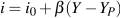
, which reflects the central bank's estimate of the size of the effect of an interest rate change on aggregate expenditure.

Figure 10.5 shows how this policy rule works. In Panel a), output is measured on the horizontal axis and interest rates on the vertical axis. A vertical line is drawn at the potential output level Y_P. The positively sloped line showing the central bank's reaction to fluctuations in output crosses the Y_P line at the interest rate i₀ with a slope of . If output were lower than Y_P, at Y₁ for example, the bank would lower interest rates to i₁ to provide some stimulus to aggregate expenditure.

Figure 10.5 Interest rates and output with a simple monetary policy rule

a) Central bank sets interest rate i₀ consistent with Y_P. changes i with a set range. Slope of line defines central bank reaction to temporary . b) A fall in A(i) causes recessionary fluctuation in Y to Y₁. Bank reacts, allowing i<i₁. Lower i increases A(i) to restore AE and equilibrium Y=Y_P. If decline in A is persistent and not offset by small fall in i the Bank will reset its target rate.

Alternatively, for an output greater than Y_P, the central bank would raise interest rates to reduce aggregate expenditure. This simple policy rule describes how the central bank resets its interest rate to achieve the target of equilibrium output at Y_P, and reacts to offset or moderate temporary fluctuations about Y_P.

Panel b) shows the effect of the changes in interest rates on equilibrium output. We studied the transmission mechanism from interest rate changes to expenditure changes in Chapter 9. The central bank chooses the interest rate i₀ that gives aggregate expenditure and equilibrium output at Y_P.

. Y would fall to Y₁, which is less than Y_P. From the monetary policy rule in Panel a), we see the reaction of the central bank. It lowers the interest rate to i₁. Lower interest rates work through the cost of and availability of finance, wealth effects, and exchange rate effects to increase expenditure. The AE line shifts back up to to restore equilibrium at Y_P. By reacting to temporary changes in the state of the economy, the central bank attempts to stabilize output at Y_P.

Figure 10.5 sets an interest rate target i₀ based on an assessment of the fundamental conditions in the economy that underlie potential output. It calls for changes in the interest rate in response to temporary fluctuations in those conditions. A more lasting change in economic conditions would need a different policy rule. Changes in the Bank of Canada's overnight interest rate in 2015 in response to falling oil and commodity prices provide an example. The central bank would choose an interest rate target different from i₀, and appropriate to equilibrium at Y_P in the new conditions. A more expansionary monetary policy at each output level would mean a target rate lower than i₀. The policy rule line in Panel a) would shift down to cross the vertical line at Y_P at the new lower target rate. A more restrictive policy would shift the line vertically up. Changes in the overnight rate in Canada or the federal funds rate in the United States are announced to tell financial markets of these changes in monetary policy.

Policy rules and inflation

The assumption that prices are constant ignores the importance of inflation, making a policy rule based on the output gap alone too simple. Central banks today, like the Bank of Canada, conduct their monetary policy by setting inflation targets. This does not mean that they ignore the level of output in the economy. Instead, inflationary and recessionary gaps, and changes in unemployment rates, are seen as important predictors of future inflation. The simple monetary policy rule of Equation 10.1 is easily extended to recognize this current approach to monetary policy.

The central bank's setting of its interest rate instrument could then be:

1. (i₀) the interest consistent with equilibrium at potential output (Y_P) plus an adjustment to that rate if:
2. () the current inflation rate differs from , the Bank's inflation rate target plus a second adjustment if:
3. (Y–Y_P) the output gap does not equal zero.

This gives a basic equation that describes the central bank's policy reaction to economic conditions.

(10.2)

As before, the central bank sets an interest rate i₀. This is the nominal interest rate the bank thinks is consistent with output at potential output and inflation at the target rate under current conditions.

The Bank of Canada's current inflation target, for example, is percent, the midpoint of a 1 percent to 3 percent range. If inflation rises above the target , the central bank raises the nominal interest rate. The parameter a in the equation tells us by how much the nominal interest rate is changed in response to an inflation rate different from the bank's target.

Expenditure decisions depend on the interest rate. To stick to its inflation target, the bank must change the interest rate by changing the nominal interest rate by more than any change in inflation. This requires the parameter a>1. A rise in inflation is then met by a rise in interest rates that is large enough to reduce expenditure and inflationary pressure.

By this rule, the central bank also reacts to any departure of output from potential output, as it did in our earlier study of the simple rule, Equation 10.1. The parameter measures how much the central bank would raise the interest rate in response to an inflationary gap, or lower it in response to a recessionary gap. Output stabilization requires that interest rates be raised in the case of an inflationary gap or lowered in the case of a recessionary gap thus is greater than zero ().

Changing interest rates to offset an output gap is intended to stabilize output, but it will also work to offset any changes in the future inflation rate that would be caused by a persistent output gap. The size of the central bank's reactions, as measured by the parameters a and are indications of the relative importance it attaches to inflation control and output stabilization.

Any change in economic conditions that the central bank thinks is going to last for some time will result in a change in its setting of i₀. The policy line in a diagram would shift up or down. Interest rates would then be higher or lower for all inflation rates and output gaps, depending on the change in i₀. The central bank would announce this change in the setting of its policy instrument, the overnight rate in Canada or the federal funds rate in the United States. Bank of Canada press releases explain overnight rate settings. See for example:

http://www.bankofcanada.ca/2017/04/fad-press-release-2017-04-12/

This approach to monetary policy has similarities to our earlier discussion of fiscal policy. In that case, we distinguished between automatic and discretionary policy. In the case of monetary policy, the discretionary component is the setting of the operating range for the overnight rate. These decisions are based on an evaluation of longer-term economic conditions relative to the target inflation rate. It positions the monetary policy line in a diagram in much the same way as the structural budget balance positions the government's BB line in Chapter 7. Short-term fluctuations in economic conditions result in short-term variations in the overnight rate—movements along the monetary policy line. This is similar to the automatic stabilization that comes from movements along the government's BB line as a result of fluctuations in output and income.

There is, however, an important difference between monetary and fiscal policy. Monetary policy that uses the interest rate as the policy instrument provides strong automatic stabilization in response to money and financial market disturbances. Automatic stabilization in fiscal policy reduces the effects of fluctuations in autonomous expenditures.

The effective lower bound (ELB)

The financial crisis and recession of 2008-09 led to new and more intense monetary policy actions by central banks. Most continued with cuts to basic policy rates as their first response. The Federal Reserve in the United States lowered its federal funds rate, in steps, to a range of zero to 0.25 percent. The Bank of Canada followed, lowering its overnight rate setting to 0.5 percent by early March 2009. But these lower rates were not sufficient to stimulate borrowing and expenditure. Banks and other lenders were concerned by the increased risks of losses on their current lending and the risks involved in new lending. They had suffered losses on previous large denomination fixed term and mortgage lending. Bankruptcies were rising across many business and consumer loan markets.

With their policy interest rates cut to near zero, central banks hit the effective lower bound (ELB). Nominal interest rates could not be reduced any further. Central banks needed additional policy tools to meet deep concerns about risk and liquidity in financial markets. Increased demands for liquidity raised desired reserve and currency holdings and lowered money supply multipliers in many countries, and restricted access to bank credit.

Effective lower bound (ELB): A Bank's policy interest rate cannot be set below a small positive number.

Two previously used techniques were introduced. The first was increased "moral suasion," an increase in communications with financial market participants to emphasize the central bank's longer-term support for markets and its actions to promote stability. More directly the banks were urged to maintain their lending operations.

Moral suasion: a central bank persuades and encourages banks to follow its policy initiatives and guidance.

The second was "quantitative easing," and in the case of the US, an even more extensive "credit easing." "Quantitative easing" is the large scale purchase of government securities on the open market. It expands the central bank's balance sheet and the size of the monetary base. A version of this policy action was used in Japan earlier in the decade after the Bank of Japan had lowered its borrowing rate to zero and wanted to provide further economic stimulus.

Quantitative easing: a large scale purchase of government securities to increase the monetary base.

Credit easing is measured by the expanded variety of loans and securities the central bank willingly holds on its balance sheet. These come from purchases of private sector assets in certain troubled credit markets. The mortgage market for example was in trouble as a result of falling real estate prices and mortgage defaults. Cash is put directly into specific markets rather than letting it feed it through commercial banks' lending and loan portfolio decisions.

Credit easing: the management of the central bank's assets designed to support lending in specific financial markets.

Monetary policy practice continues to evolve. In the last few years, with policy interest rates at or near the effective lower bound and persistent weakness in economic growth and employment, major central banks have relied increasingly on "forward guidance" to support their economies. Forward guidance is contained in the explanation a Bank gives in its formal announcement of setting of the policy interest rate. If for example the Bank's opinion that economic growth and inflation will be slow and weak, the Bank suggests that interest rates will be unchanged for some time into the future. Alternatively a prediction of a revival in growth and inflationary pressure may lead the Bank to predict increases in policy interest rates in the near future.

Forward guidance: information on the timing of future changes in the central bank's interest rate setting.

This forward guidance is intended to help firms and households make expenditure decisions that require debt financing. In some cases it is based on an explicit economic criterion.

For example, the US and the UK recently introduced unemployment rate thresholds for changes in the monetary policy rate settings. This is in essence a variety of forward guidance. In the UK, for example, in August 2013 the Bank of England, under the heading "Forward Guidance" announced:

In particular, the MPC [Monetary Policy Committee] intends not to raise Bank Rate from its current level of 0.5% at least until the Labour Force Survey headline measure of the unemployment rate has fallen to a threshold of 7%, subject to the conditions below.

Source:

www.bankofengland.co.uk/monetarypolicy/pages/forwardguidance.aspx

In effect, putting an unemployment rate target into the interest rate setting rule is a variation on the rule specified by Equation 10.2. It adds to or replaces the output gap target with an unemployment rate target.