5.1 Equity and efficiency
In modern mixed economies, markets and governments together determine the
output produced and also who benefits from that output. In this chapter we
explore a very broad question that forms the core of welfare economics: Even if market forces drive efficiency, are they a good way to allocate scarce resources in view of the fact that
they not only give rise to inequality and poverty, but also fail to capture
the impacts of productive activity on non-market participants? Mining
impacts the environment, traffic results in road fatalities, alcohol, tobacco and opioids cause premature deaths. These
products all generate secondary impacts beyond their stated objective. We
frequently call these external effects.
The analysis of markets in this
larger sense involves not just economic efficiency; public policy
additionally has a normative content because policies can impact the various
participants in different ways and to different degrees. Welfare economics, therefore, deals with both normative and
positive issues.
Welfare economics assesses how well the economy allocates its scarce resources in accordance with the goals of efficiency and equity.
Political parties on the left and right disagree on how well a market
economy works. Canada's New Democratic Party emphasizes the market's
failings and the need for government intervention, while the Progressive
Conservative Party believes, broadly, that the market fosters choice,
incentives, and efficiency. What lies behind this disagreement? The two
principal factors are efficiency and equity.
Efficiency addresses the question of how well the economy's resources are
used and allocated. In contrast, equity deals with how society's goods and
rewards are, and should be, distributed among its different members, and how
the associated costs should be apportioned.
Equity deals with how society's goods and rewards are, and should be, distributed among its different members, and how the associated costs should be apportioned.
Efficiency addresses the question of how well the economy's resources are used and allocated.
Equity is also concerned with how different generations share an economy's
productive capabilities: More investment today makes for a more productive
economy tomorrow, but more greenhouse gases today will reduce environmental
quality tomorrow. These are inter-generational questions.
Climate change caused by global warming forms one of the biggest challenges
for humankind at the present time. As we shall see in this chapter,
economics has much to say about appropriate policies to combat warming.
Whether pollution-abatement policies should be implemented today or down the
road involves considerations of equity between generations. Our first task
is to develop an analytical tool which will prove vital in assessing and
computing welfare benefits and costs – economic surplus.
5.2 Consumer and producer surplus
An understanding of economic efficiency is greatly facilitated as a result
of understanding two related measures: Consumer surplus and producer
surplus. Consumer surplus relates to the demand side of the market, producer
surplus to the supply side. Producer surplus is also termed supplier
surplus. These measures can be understood with the help of a standard
example, the market for city apartments.
The market for apartments
Table 5.1 and Figure 5.1
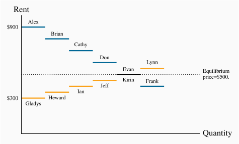
describe the hypothetical data. We imagine first a series of city-based
students who are in the market for a standardized downtown apartment. These
individuals are not identical; they value the apartment differently. For
example, Alex enjoys comfort and therefore places a higher value on a unit
than Brian. Brian, in turn, values it more highly than Cathy or Don. Evan
and Frank would prefer to spend their money on entertainment, and so on.
These valuations are represented in the middle column of the demand panel in
Table 5.1, and also in Figure 5.1
with the highest valuations closest to the origin. The valuations reflect
the willingness to pay of each consumer.
Table 5.1 Consumer and supplier surpluses
|
Demand |
|
Individual | Demand valuation | Surplus |
|
Alex | 900 | 400 |
|
Brian | 800 | 300 |
|
Cathy | 700 | 200 |
|
Don | 600 | 100 |
|
Evan | 500 | 0 |
|
Frank | 400 | 0 |
|
|
|
Supply |
|
Individual | Reservation value | Surplus |
|
Gladys | 300 | 200 |
|
Heward | 350 | 150 |
|
Ian | 400 | 100 |
|
Jeff | 450 | 50 |
|
Kirin | 500 | 0 |
|
Lynn | 550 | 0 |
On the supply side we imagine the market as being made up of different
individuals or owners, who are willing to put their apartments on the market
for different prices. Gladys will accept less rent than Heward, who in turn
will accept less than Ian. The minimum prices that the suppliers are willing
to accept are called reservation prices or values, and these are
given in the lower part of Table 5.1. Unless the
market price is greater than their reservation price, suppliers will hold
back.
By definition, as stated in Chapter 3, the demand curve
is made up of the valuations placed on the good by the various demanders.
Likewise, the reservation values of the suppliers form the supply curve. If
Alex is willing to pay $900, then that is his demand price; if Heward is
willing to put his apartment on the market for $350, he is by definition
willing to supply it for that price. Figure 5.1
therefore describes the demand and supply curves in this market. The steps
reflect the willingness to pay of the buyers and the reservation valuations
or prices of the suppliers.
In this example, the equilibrium price for apartments will be $500. Let us
see why. At that price the value placed on the marginal unit supplied by
Kirin equals Evan's willingness to pay. Five apartments will be rented. A
sixth apartment will not be rented because Lynn will let her apartment only
if the price reaches $550. But the sixth potential demander is willing to
pay only $400. Note that, as usual, there is just a single price in the
market. Each renter pays $500, and therefore each supplier also receives
$500.
The consumer and supplier surpluses can now be computed. Note that, while
Don is willing to pay $600, he actually pays $500. His consumer surplus is
therefore $100. In Figure 5.1, we can see that each consumer's surplus is the distance between the market price
and the individual's valuation. These values are given in the final column
of the top half of Table 5.1.
Consumer surplus is the excess of consumer willingness to pay over the market price.
Using the same reasoning, we can compute each supplier's
surplus, which is the excess of the amount obtained for the rented
apartment over the reservation price. For example, Heward obtains a surplus
on the supply side of $150, while Jeff gets $50. Heward is willing to put
his apartment on the market for $350, but gets the equilibrium price/rent
of $500 for it. Hence his surplus is $150.
Supplier or producer surplus is the excess of market price over the reservation price of the supplier.
It should now be clear why these measures are called surpluses. The
suppliers and demanders are all willing to participate in this market
because they earn this surplus. It is a measure of their gain from being
involved in the trading. The sum of each participant's surplus in the final
column of Table 5.1 defines the total surplus in the
market. Hence, on the demand side a total surplus arises of $1,000 and on
the supply side a value of $500.
The taxi market
We do not normally think of demand and supply functions in terms of the
steps illustrated in Figure 5.1. Usually there are so
many participants in the market that the differences in reservation prices
on the supply side and willingness to pay on the demand side are exceedingly
small, and so the demand and supply curves are drawn as continuous lines. So
our second example reflects this, and comes from the market for taxi rides.
We might think of this as an Uber- or Lyft-type taxi operation.
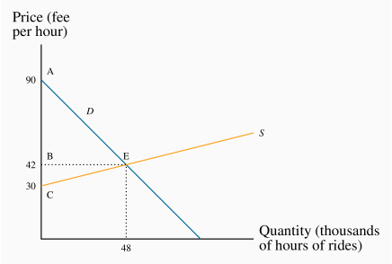
Let us suppose that the demand and supply curves for taxi rides in a given
city are given by the functions in Figure 5.2.
The demand curve represents
the willingness to pay on the part of riders. The supply curve represents
the willingness to supply on the part of drivers. The price per hour of
rides defines the vertical axis; hours of rides (in thousands) are measured on the
horizontal axis. The demand intercept of $90 says that the person who
values the ride most highly is willing to pay $90 per hour. The downward
slope of the demand curve states that other buyers are willing to pay less.
On the supply side no driver is willing to supply his time and vehicle
unless he obtains at least $30 per hour. To induce additional suppliers a
higher price must be paid, and this is represented by the upward sloping
supply curve.
The intersection occurs at a price of $42 per hour and the equilibrium
number of ride-hours supplied is 48 thousand.
Computing the surpluses is very straightforward. By definition the consumer
surplus is the excess of the willingness to pay by each buyer above the
uniform price. Buyers who value the ride most highly obtain the biggest
surplus – the highest valuation rider gets a surplus of $48 per hour – the
difference between his willingness to pay of $90 and the actual price of
$42. Each successive rider gets a slightly lower surplus until the final
rider, who obtains zero. She pays $42 and values the ride hours at $42
also. On the supply side, the drivers who are willing to supply rides at the
lowest reservation price ($30 and above) obtain the biggest surplus. The
'marginal' supplier gets no surplus, because the price equals her
reservation price.
From this discussion it follows that the consumer surplus is given by the
area ABE and the supplier surplus by the area CBE. These are two
triangular areas, and measured as half of the base by the perpendicular
height. Therefore, in thousands of units:
The total surplus that arises in the market is the sum of producer and
consumer surpluses, and since the units are in thousands of hours the total
surplus here is  .
.
5.3 Efficient market outcomes
The definition and measurement of the surplus is straightforward
provided the supply and demand functions are known. An important
characteristic of the marketplace is that in certain circumstances it
produces what we call an efficient outcome, or an efficient
market. Such an outcome yields the highest possible sum of surpluses.
An efficient market maximizes the sum of producer and consumer surpluses.
To see that this outcome achieves the goal of maximizing the total surplus,
consider what would happen if the quantity Q=48 in the taxi example were not supplied. Suppose
that the city's taxi czar decreed that 50 units should be supplied, and
the czar forced additional drivers on the road. If 2 additional units are
to be traded in the market, consider the value of this at the margin.
Suppliers value the supply more highly than the buyers are willing to pay.
So on these additional 2 units negative surplus would accrue, thus
reducing the total.
A second characteristic of the market equilibrium is that potential buyers who would like a cheaper ride and drivers who would
like a higher hourly payment do not participate in the market. On the
demand side those individuals who are unwilling to pay $42/hour can take public transit, and on the supply
side the those drivers who are unwilling to supply at $42/hour can allocate their time to alternative activities.
Obviously, only those who participate in the market benefit from a surplus.
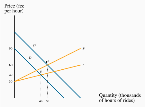
One final characteristic of surplus measurement should be emphasized. That
is, the surplus number is not unique, it depends upon the economic
environment. We can illustrate this easily using the taxi example. A well
recognized feature of Uber taxi rides is that the price varies with road and
weather conditions. Poor weather conditions mean that there is an increased
demand, and poor road or weather conditions mean that drivers are less
willing to supply their services – their reservation payment increases. This
situation is illustrated in Figure 5.3.
The demand curve has shifted
upwards and the supply curve has also changed in such a way that any
quantity will now be supplied at a higher price. The new equilibrium is
given by  rather than E. There is a new equilibrium
price-quantity combination that is efficient in the new market
conditions. This illustrates that there is no such thing as a unique
unchanging efficient outcome. When economic factors that influence the
buyers' valuations (demand) or the suppliers' reservation prices (supply)
change, then the efficient market outcome must be recomputed.
rather than E. There is a new equilibrium
price-quantity combination that is efficient in the new market
conditions. This illustrates that there is no such thing as a unique
unchanging efficient outcome. When economic factors that influence the
buyers' valuations (demand) or the suppliers' reservation prices (supply)
change, then the efficient market outcome must be recomputed.
5.4 Taxation, surplus and efficiency
Despite enormous public interest in taxation and its impact on the economy,
it is one of the least understood areas of public policy. In this section we
will show how an understanding of two fundamental tools of
analysis – elasticities and economic surplus – provides powerful insights
into the field of taxation.
We begin with the simplest of cases: The federal government's goods and
services tax (GST) or the provincial governments' sales taxes (PST). These
taxes combined vary by province, but we suppose that a typical rate is 13
percent. In some provinces these two taxes are harmonized. Note that
this is a percentage, or ad valorem,
tax, not a specific tax of so many dollars per unit traded.
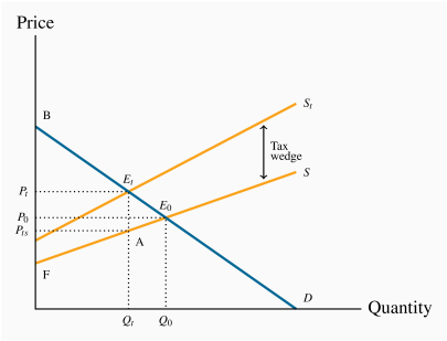
Figure
5.4 illustrates the supply and demand curves for
some commodity. In the absence of taxes, the equilibrium E0 is defined by
the combination (P0, Q0).
A 13-percent tax is now imposed, and the new supply curve St lies 13
percent above the no-tax supply S. A tax wedge is therefore
imposed between the price the consumer must pay and the price that the
supplier receives. The new equilibrium is Et, and the new market price is
at Pt. The price received by the supplier is lower than that paid by the
buyer by the amount of the tax wedge. The post-tax supply price is denoted
by  .
.
There are two burdens associated with this tax. The first is the revenue burden, the amount of tax revenue paid by the market
participants and received by the government. On each of the Qt units
sold, the government receives the amount  . Therefore, tax
revenue is the amount
. Therefore, tax
revenue is the amount  A. As illustrated in Chapter 4,
the degree to which the market price Pt rises
above the no-tax price P0 depends on the supply and demand elasticities.
A. As illustrated in Chapter 4,
the degree to which the market price Pt rises
above the no-tax price P0 depends on the supply and demand elasticities.
A tax wedge is the difference between the consumer and producer prices.
The revenue burden is the amount of tax revenue raised by a tax.
The second burden of the tax is called the excess burden. The
concepts of consumer and producer surpluses help us comprehend this. The
effect of the tax has been to reduce consumer surplus by  . This is the reduction in the pre-tax surplus given by
the triangle
. This is the reduction in the pre-tax surplus given by
the triangle  B
B . By the same reasoning, supplier surplus is
reduced by the amount
. By the same reasoning, supplier surplus is
reduced by the amount  A; prior to the tax it was
  . Consumers and suppliers have therefore seen a reduction in
their well-being that is measured by these dollar amounts. Nonetheless, the
government has additional revenues amounting to A, and
this tax imposition therefore represents a transfer from the
consumers and suppliers in the marketplace to the government. Ultimately,
the citizens should benefit from this revenue when it is used by the
government, and it is therefore not considered to be a net loss of surplus.
. Consumers and suppliers have therefore seen a reduction in
their well-being that is measured by these dollar amounts. Nonetheless, the
government has additional revenues amounting to A, and
this tax imposition therefore represents a transfer from the
consumers and suppliers in the marketplace to the government. Ultimately,
the citizens should benefit from this revenue when it is used by the
government, and it is therefore not considered to be a net loss of surplus.
However, there remains a part of the surplus loss that is not transferred,
the triangular area  A. This component is called the excess burden, for the reason that it represents the component
of the economic surplus that is not transferred to the government in the
form of tax revenue. It is also called the deadweight loss,
DWL.
A. This component is called the excess burden, for the reason that it represents the component
of the economic surplus that is not transferred to the government in the
form of tax revenue. It is also called the deadweight loss,
DWL.
The excess burden, or deadweight loss, of a tax is the component of consumer and producer surpluses forming a net loss to the whole economy.
The intuition behind this concept is not difficult. At the output  ,
the value placed by consumers on the last unit supplied is
,
the value placed by consumers on the last unit supplied is  (
( ),
while the production cost of that last unit is (=A). But the
potential surplus (
),
while the production cost of that last unit is (=A). But the
potential surplus ( ) associated with producing an additional
unit cannot be realized, because the tax dictates that the production
equilibrium is at rather than any higher output. Thus, if output
could be increased from to
) associated with producing an additional
unit cannot be realized, because the tax dictates that the production
equilibrium is at rather than any higher output. Thus, if output
could be increased from to  , a surplus of value over cost
would be realized on every additional unit equal to the vertical distance
between the demand and supply functions D and S. Therefore, the loss
associated with the tax is the area A.
, a surplus of value over cost
would be realized on every additional unit equal to the vertical distance
between the demand and supply functions D and S. Therefore, the loss
associated with the tax is the area A.
In public policy debates, this excess burden is rarely discussed. The reason
is that notions of consumer and producer surpluses are not well understood
by non-economists, despite the fact that the value of lost surpluses is
frequently large. Numerous studies have estimated the excess burden
associated with raising an additional dollar from the tax system. They
rarely find that the excess burden is less than 25 percent of total
expenditure. This is a sobering finding. It tells us that if the government
wished to implement a new program by raising additional tax revenue, the
benefits of the new program should be 25 percent greater than the amount
expended on it!
The impact of taxes and other influences that result in an inefficient use
of the economy's resources are frequently called distortions
because they necessarily lead the economy away from the efficient output.
The magnitude of the excess burden is determined by the elasticities of
supply and demand in the markets where taxes are levied. To see this, return
to Figure 5.4, and suppose that the demand curve
through E0 were more elastic (with the same supply curve, for
simplicity). The post-tax equilibrium Et would now yield a lower Qt
value and a price between Pt and P0. The resulting tax revenue
raised and the magnitude of the excess burden would differ because of the
new elasticity.
A distortion in resource allocation means that production is not at an efficient output.
5.5 Market failures – externalities
The consumer and producer surplus concepts we have developed are extremely
powerful tools of analysis, but the world is not always quite as
straightforward as simple models indicate. For example, many suppliers
generate pollutants that adversely affect the health of the population, or
damage the environment, or both. The term externality is used
to denote such impacts. Externalities impact individuals who are not
participants in the market in question, and the effects of the externalities
may not be captured in the market price. For example, electricity-generating
plants that use coal reduce air quality, which, in turn, adversely impacts
individuals who suffer from asthma or other lung ailments. While this is an
example of a negative externality, externalities can also be positive.
An externality is a benefit or cost falling on people other than those involved in the activity's market. It can create a difference between private costs or values and social costs or values.
We will now show why markets characterized by externalities are not
efficient, and also show how these externalities might be corrected or
reduced. The essence of an externality is that it creates a divergence
between private costs/benefits and social costs/benefits. If a steel
producer pollutes the air, and the steel buyer pays only the costs incurred
by the producer, then the buyer is not paying the full "social" cost of
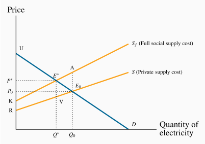
the product. The problem is illustrated in Figure 5.5.
Negative externalities
In Figure 5.5, the supply curve S represents the cost to
the supplier, whereas Sf (the full cost) reflects, in
addition, the cost of bad air to the population. Of course, we are assuming
that this external cost is ascertainable, in order to be able to
characterize Sf accurately. Note also that this illustration assumes
that, as power output increases, the external cost per unit rises,
because the difference between the two supply curves increases with output.
This implies that low levels of pollution do less damage per unit: Perhaps
the population has a natural tolerance for low levels, but higher levels
cannot be tolerated easily and so the cost per unit is greater.
Despite the externality, an efficient level of production can still
be defined. It is given by Q×, not Q0. To see why, consider the
impact of reducing output by one unit from Q0. At Q0 the willingness
of buyers to pay for the marginal unit supplied is E0. The (private)
supply cost is also E0. But from a societal standpoint there is a
pollution/health cost of AE0 associated with that unit of production. The
full cost, as represented by Sf, exceeds the buyer's valuation.
Accordingly, if the last unit of output produced is cut, society gains by
the amount AE0, because the cut in output reduces the excess of true cost
over value.
Applying this logic to each unit of output between Q0 and Q×, it is
evident that society can increase its well-being by the dollar amount equal
to the area E×AE0, as a result of reducing production.
Next, consider the consequences of reducing output further from Q×.
Note that some pollution is being created here, and environmentalists
frequently advocate that pollution should be reduced to zero. However, an
efficient outcome may not involve a zero level of pollution! If the
production of power were reduced below Q×, the loss in value to
buyers, as a result of not being able to purchase the good, would exceed the
full cost of its production.
If the government decreed that, instead of producing Q×, no pollution
would be tolerated, then society would forgo the possibility of earning the
total real surplus equal to the area UE×K. Economists do not advocate
such a zero-pollution policy; rather, we advocate a policy that permits a
"tolerable" pollution level – one that still results in net benefits to
society. In this particular example, the total cost of the tolerated
pollution equals the area between the private and full supply functions, KE×VR.
As a matter of policy, how is this market influenced to produce the amount Q× rather than Q0? One option would be for the government to intervene
directly with production quotas for each firm. An alternative would be to
impose a corrective tax on the good whose production causes
the externality: With an appropriate increase in the price, consumers will
demand a reduced quantity. In Figure 5.5 a tax equal to
the dollar value VE× would shift the supply curve upward by that amount
and result in the quantity Q× being traded.
A corrective tax seeks to direct the market towards a more efficient output.
We are now venturing into the field of environmental policy, where a corrective tax is usually called a carbon tax, and this is
explored in the following section. The key conclusion of the foregoing
analysis is that an efficient working of the market continues to have
meaning in the presence of externalities. An efficient output level still
maximizes economic surplus where surplus is correctly defined.
Positive externalities
Externalities of the positive kind enable individuals or producers
to get a type of 'free ride' on the efforts of others. Real world examples
abound: When a large segment of the population is immunized against
disease, the remaining individuals benefit on account of the reduced
probability of transmission.
A less well recognized example is the benefit derived by many producers
world-wide from research and development (R&D) undertaken in advanced
economies and in universities and research institutes. The result is that
society at large, including the corporate sector, gain from this enhanced
understanding of science, the environment, or social behaviours.
The free market may not cope any better with these positive externalities
than it does with negative externalities, and government intervention may be
beneficial. Furthermore, firms that invest heavily in research and
development would not undertake such investment if competitors could have a
complete free ride and appropriate the fruits. This is why patent
laws exist, as we shall see later in discussing Canada's competition
policy. These laws prevent competitors from copying the product development
of firms that invest in R&D. If such protection were not in place, firms
would not allocate sufficient resources to R&D, which is a real engine of
economic growth. In essence, the economy's research-directed resources would
not be appropriately rewarded, and thus too little research would take place.
While patent protection is one form of corrective action, subsidies are
another. We illustrated above that an appropriately formulated tax on a good
that creates negative externalities can reduce demand for that good, and
thereby reduce pollution. A subsidy can be thought of as a negative tax, and
can stimulate the supply of goods and services that have positive
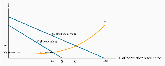
externalities. Consider the example in Figure 5.6.
Individuals have a demand for flu shots given by D. This reflects their
private valuation – their personal willingness to pay. But the social value
of flu shots is greater. When more individuals are vaccinated,
the probability that others will be infected falls. Additionally, with
higher rates of immunization, the health system will incur fewer costs in
treating the infected. Therefore, the value to society of any quantity of
flu shots is greater than the sum of the values that individuals place on
them.
Df reflects the full social value of any quantity of flu shots. In this instance the quantity axis measures the percentage of the population vaccinated, which has a maximum of 100%. If S is the supply curve, the socially optimal, efficient, market outcome is
Q×. The steeply upward-sloping section of S denotes that it may be very costly to vaccinate every last person – particularly those living in outlying communities. How can we influence the market to move from Q0 towards Q×?
One solution is a subsidy that would reduce the price to zero. In this case that gets us almost to the optimum, because the percentage of the population now choosing to be vaccinated is given by  . The zero price essentially makes the supply curve, as perceived by the population, to be running along the horizontal axis.
Note the social value of the improvement in moving from Q0 to ; the social value exceeds the social cost. But even at further gains are available because at the social value of additional vaccinations is greater than the social cost. Overall, at the point Q× the social value is given by the area under the demand curve, and the social cost by the area under the supply curve.
5.7 Environmental policy and climate change
Greenhouse gases
The greatest externality challenge in the modern world is to control our
emissions of greenhouse gases.The emission of greenhouse gases
(GHGs) is associated with a wide variety of economic activities such as
coal-based power generation, oil-burning motors, wood-burning stoves, ruminant animals, etc.
The most common GHG is carbon dioxide, methane is another. The gases, upon emission, circulate
in the earth's atmosphere and, following an excessive build-up, prevent
sufficient radiant heat from escaping. The result is a slow warming of the
earth's surface and air temperatures. It is envisaged that such temperature
increases will, in the long term, increase water temperatures and cause glacial melting, with the result that water levels worldwide will
rise. In addition to the higher water levels, which the Intergovernmental
Panel on Climate Change (IPCC) estimates will be between one foot and one
metre by the end of the 21st century, oceans will become
more acidic, weather patterns will change and weather events become more
variable and severe. The changes will be latitude-specific and vary by
economy and continent, and ultimately will impact the agricultural
production abilities of certain economies.
Greenhouse gases that accumulate excessively in the earth's atmosphere prevent heat from escaping and lead to global warming.
While most scientific findings and predictions are subject to a degree of
uncertainty, there is little disagreement in the scientific community on the long-term impact of increasing GHGs in the atmosphere. There is some
skepticism as to whether the generally higher temperatures experienced in
recent decades are completely attributable to anthropogenic activity since
the industrial revolution, or whether they also reflect a natural cycle in
the earth's temperature. But scientists agree that a continuance of the
recent rate of GHG emissions is leading to serious climatic
problems.
The major economic environmental challenge facing the world economy is this: Historically, GHG emissions have been strongly correlated with economic growth. The very high rate of economic growth in many large-population economies such as China and India that will be necessary to raise hundreds of millions out of poverty means that that historical pattern needs to be broken – GHG accumulation must be "decoupled" from economic growth.
GHGs as a common property
A critical characteristic of GHGs is that they are what we call in economics
a 'common property': Every citizen in the world 'owns' them, every citizen
has equal access to them, and it matters little where these GHGs originate.
Consequently, if economy A reduces its GHG emissions, economy B may simply
increase its emissions rather than incur the cost of reducing them. Hence,
economy A's behaviour goes unrewarded. This is the crux of international
agreements – or disagreements. Since GHGs are a common property, in order
for A to have the incentive to reduce emissions, it needs to know that B
will act correspondingly.
From the Kyoto Protocol to the Paris Accord
The world's first major response to climate concerns came in the form of the
United Nations–sponsored Earth Summit in Rio de Janeiro in 1992. This was
followed by the signing of the Kyoto Protocol in 1997, in which a group of
countries committed themselves to reducing their GHG emissions relative to
their 1990 emissions levels by the year 2012. Canada's Parliament
subsequently ratified the Kyoto Protocol, and thereby agreed to meet
Canada's target of a 6 percent reduction in GHGs relative to the amount
emitted in 1990.
On a per-capita basis, Canada is one of the world's largest contributors to
global warming, even though Canada's percentage of the total is just 2
percent. Many of the world's major economies refrained from signing the
Protocol—most notably China, the United States, and India. Canada's
emissions in 1990 amounted to approximately 600 giga tonnes (Gt) of carbon
dioxide; but by the time we ratified the treaty in 2002, emissions were 25%
above that level. Hence the signing was somewhat meaningless, in that Canada
had virtually a zero possibility of attaining its target.
The target date of 2012 has come and gone and subsequent conferences in
Copenhagen and Rio failed to yield an international agreement. But in Paris,
December 2015, 195 economies committed to reduce their GHG emissions by
specific amounts. Canada was a party to that agreement. Target reductions
varied by country. Canada committed itself to reduce GHG emissions by 30% by
the year 2030 relative to 2005 emissions levels. To this end the Liberal
government of Prime Minister Justin Trudeau announced in late 2016 that if
individual Canadian provinces failed to implement a carbon tax, or
equivalent, the federal government would impose one unilaterally. The program involves a carbon tax of $10 per tonne in 2018, that increases by $10 per annum until it attains a value of $50 in 2022. Some provinces already have GHG limitation
systems in place (cap and trade systems - developed below), and these
provinces would not be subject to the federal carbon tax provided the
province-level limitation is equivalent to the federal carbon tax.
Canada's GHG emissions
An excellent summary source of data on Canada's emissions and performance
during the period 1990-2018 is available on Environment Canada's web site.
See:
www.canada.ca/en/environment-climate-change/services/climate-change/greenhouse-gas-emissions/sources-sinks-executive-summary-2020.html#toc3
Canada, like many economies, has become more efficient in its use of energy
(the main source of GHGs) in recent decades—its use of energy per
unit of total output has declined steadily. Canada emitted 0.44 mega tonnes of  equivalent per billion dollars of GDP in 2005, and 0.36 mega tonnes in 2017. On a per capita basis
Canada's emissions amounted to 22.9 tonnes in 2005, and dropped to 19.5 by
2017. This modest improvement in efficiency means that Canada's GDP is now less energy intensive. The critical challenge is
to produce more output while using not just less energy per unit of output,
but to use less energy in total.
equivalent per billion dollars of GDP in 2005, and 0.36 mega tonnes in 2017. On a per capita basis
Canada's emissions amounted to 22.9 tonnes in 2005, and dropped to 19.5 by
2017. This modest improvement in efficiency means that Canada's GDP is now less energy intensive. The critical challenge is
to produce more output while using not just less energy per unit of output,
but to use less energy in total.
While Canada's energy intensity (GHGs per unit of output) has dropped, overall emissions have increased by almost 20% since 1990. Furthermore,
while developed economies have increased their efficiency, it is the world's efficiency that is ultimately critical. By outsourcing much of its
manufacturing sector to China, Canada and the West have offloaded some of
their most GHG-intensive activities. But GHGs are a common property resource.
Canada's GHG emissions also have a regional aspect: The production
of oil and gas, which has created considerable wealth for all Canadians, is
both energy intensive and concentrated in a limited number of provinces
(Alberta, Saskatchewan and more recently Newfoundland and Labrador).
GHG measurement
GHG atmospheric concentrations are measured in parts per million (ppm).
Current levels in the atmosphere are slightly above 400 ppm, and continued growth in
concentration will lead to serious economic and social disruption. In the
immediate pre-industrial revolution era concentrations were in the 280 ppm
range. Hence, our world seems to be headed towards a doubling of GHG concentrations in the coming decades.
GHGs are augmented by the annual additions to the stock already in the
atmosphere, and at the same time they decay—though very slowly.
GHG-reduction strategies that propose an immediate reduction in emissions
are more costly than those aimed at a more gradual reduction. For example, a
slower investment strategy would permit in-place production and
transportation equipment to reach the end of its economic life rather than
be scrapped and replaced 'prematurely'. Policies that focus upon longer-term
replacement are therefore less costly in this specific sense.
While not all economists and policy makers agree on the time scale for
attacking the problem, the longer that GHG reduction is postponed, the
greater the efforts will have to be in the long term—because GHGs will
build up more rapidly in the near term.
A critical question in controlling GHG emissions relates to the cost of
their control: How much of annual growth might need to be sacrificed in
order to get emissions onto a sustainable path? Again estimates vary. The
Stern Review (2006) proposed that, with an increase in technological
capabilities, a strategy that focuses on the relative near-term
implementation of GHG reduction measures might cost "only" a few
percentage points of the value of world output. If correct, this is a low
price to pay for risk avoidance in the longer term.
Nonetheless, such a reduction will require particular economic policies, and
specific sectors will be impacted more than others.
Economic policies for climate change
There are three main ways in which polluters can be controlled. One involves
issuing direct controls; the other two involve incentives—in the form of
pollution taxes, or on tradable "permits" to pollute.
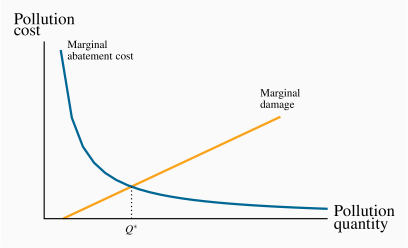
To see how these different policies operate, consider first Figure 5.7. It is a standard diagram in environmental economics,
and is somewhat similar to our supply and demand curves. On the horizontal
axis is measured the quantity of environmental damage or pollution, and on
the vertical axis its dollar value or cost. The upward-sloping damage curve
represents the cost to society of each additional unit of pollution or gas,
and it is therefore called a marginal damage curve. It is
positively sloped to reflect the reality that, at low levels of emissions,
the damage of one more unit is less than at higher levels. In terms of our
earlier discussion, this means that an increase in GHGs of 10 ppm when
concentrations are at 300 ppm may be less damaging than a corresponding
increase when concentrations are at 500 ppm.
The marginal damage curve reflects the cost to society of an additional unit of pollution.
The second curve is the abatement curve. It reflects the cost of reducing
emissions by one unit, and is therefore called a
marginal
abatement curve. This curve has a negative slope indicating that, as we
reduce the total quantity of pollution produced (moving towards the origin on the horizontal axis), the cost of further unit
reductions rises. This shape corresponds to reality. For example, halving
the emissions of pollutants and gases from automobiles may be achieved by
adding a catalytic converter and reducing the amount of lead in gasoline.
But reducing those emissions all the way to zero requires the development of
major new technologies such as electric cars—an enormously more costly
undertaking.
The marginal abatement curve reflects the cost to society of reducing the quantity of pollution by one unit.
If producers are unconstrained in the amount of pollution they produce, they
will produce more than what we will show is the optimal amount –
corresponding to Q×. This amount is optimal in the sense that at levels
greater than Q× the damage exceeds the cost of reducing the emissions.
However, reducing emissions below Q× would mean incurring a cost per unit
reduction that exceeds the benefit of that reduction. Another way of
illustrating this is to observe that at a level of pollution above Q× the
cost of reducing it is less than the damage it inflicts, and therefore a net
gain accrues to society as a result of the reduction. But to reduce
pollution below Q× would involve an abatement cost greater than the
reduction in pollution damage and therefore no net gain to society. This
constitutes a first rule in optimal pollution policy.
An optimal quantity of pollution occurs when the marginal cost of
abatement equals the marginal damage.
A second guiding principle emerges by considering a situation in which some
firms are relatively 'clean' and others are 'dirty'. More specifically, a
clean firm A may have already invested in new equipment that uses less
energy per unit of output produced, or emits fewer pollutants per unit of
output. In contrast, the dirty firm B uses older dirtier technology. Suppose
furthermore that these two firms form a particular sector of the economy and
that the government sets a limit on total pollution from this sector, and
that this limit is less than what the two firms are currently producing.
What is the least costly method to meet the target?
The intuitive answer to this question goes as follows: In order to reduce
pollution at least cost to the sector, calculate what it would cost each
firm to reduce pollution from its present level. Then implement a system so
that the firm with the least cost of reduction is the first to act. In this
case the 'dirty' firm will likely have a lower cost of abatement since it
has not yet upgraded its physical plant. This leads to a second rule in
pollution policy:
With many polluters, the least cost policy to society requires
producers with the lowest abatement costs to act first.
This principle implies that policies which impose the same emission limits
on firms may not be the least costly manner of achieving a target level of
pollution. Let us now consider the use of tradable permits and corrective/carbon taxes as policy instruments. These are
market-based systems aimed at reducing GHGs.
Tradable permits and corrective/carbon taxes are market-based systems aimed at reducing GHGs.
Incentive mechanism I: Tradable permits
A system of tradable permits is frequently called a 'cap and trade' system,
because it limits or caps the total permissible emissions, while at the same
time allows a market to develop in permits. For illustrative purposes,
consider the hypothetical two-firm sector we developed above, composed of
firms A and B. Firm A has invested in clean technology, firm B has not. Thus
it is less costly for B to reduce emissions than A if further reductions are
required. Next suppose that each firm is allocated by the government a
specific number of 'GHG emission permits'; and that the total of such
permits is less than the amount of emissions at present, and that each firm
is emitting more than its permits allow. How can these firms achieve the
target set for this sector of the economy?
The answer is that they should be able to engage in mutually beneficial
trade: If firm B has a lower cost of reducing emissions than A, then it may
be in A's interest to pay B to reduce B's emissions heavily. Imagine that
each firm is emitting 60 units of GHG, but they have permits to emit only 50
units each. And furthermore suppose it costs B $20 to reduce GHGs by one
unit, whereas it costs A $30 to do this. In this situation A could pay B
$25 for several permits and this would benefit both firms. B can reduce
GHGs at a cost of $20 and is being paid $25 to do this. In turn A would
incur a cost of $30 per unit to reduce his GHGs but he can buy permits from
B for just $25 and avoid the $30 cost. Both firms gain, and the total cost
to the economy is lower than if each firm had to reduce by the same amount.
The benefit of the cap 'n trade system is that it enables the marketplace to
reduce GHGs at least cost.
The largest system of tradable permits currently operates in the European
Union: The EU Emissions Trading System. It covers more than 10,000
large energy-using installations. Trading began in 2005. In North America a
number of Western states and several Canadian provinces are joined, either
as participants or observers, in the Western Climate Initiative,
which is committed to reduce GHGs by means of tradable emissions permits.
The longer-term goal of these systems is for the government to issue
progressively fewer permits each year, and to include an ever larger share
of GHG-emitting enterprises with the passage of time.
Policy in practice – international
In an ideal world, permits would be traded internationally, and such a
system might be of benefit to developing economies: If the cost of reducing
pollution is relatively low in developing economies because they have few
controls in place, then developed economies, for whom the cost of GA
reduction is high, could induce firms in the developing world to undertake
cost reductions. Such a trade would be mutually beneficial. For example,
imagine in the above example that B is located in the developing world and A
in the developed world. Both would obviously gain from such an arrangement,
and because GHGs are a common property, the source of GHGs from a damage
standpoint is immaterial.
Incentive mechanism II: Taxes
Corrective taxes are frequently called Pigovian taxes, after the
economist Arthur Pigou. He advocated taxing activities that cause negative
externalities. These taxes have been examined above in Section 5.4. Corrective taxes of this type can be implemented as part of a
tax package reform. For example, taxpayers are frequently reluctant
to see governments take 'yet more' of their money, in the form of new taxes.
Such concerns can be addressed by reducing taxes in other sectors of the
economy, in such a way that the package of tax changes maintains a 'revenue
neutral' impact.
Revenues from taxes and permits
Taxes and tradable permits differ in that taxes generate revenue for the
government from polluting producers, whereas permits may not generate
revenue, or may generate less revenue. If the government simply allocates permits initially to all polluters, free of charge, and allows a
market to develop, such a process generates no revenue to the government.
While economists may advocate an auction of permits in the start-up
phase of a tradable permits market, such a mechanism may run into political
objections.
Setting taxes at the appropriate level requires knowledge of the cost and
damage functions associated with GHGs. At the present time, economists and
environmental scientists think that an appropriate price or tax on one tonne
of GHG is in the  range. Such a tax would reduce emissions to a
point where the longer-term impact of GHGs would not be so severe as
otherwise.
range. Such a tax would reduce emissions to a
point where the longer-term impact of GHGs would not be so severe as
otherwise.
British Columbia introduced a carbon tax of  per tonne of GHG on fuels
in 2008, and has increased that price regularly. This tax was designed to be revenue neutral in order to make it
more acceptable. This means that British Columbia reduced its income tax
rates by an amount such that income tax payments would fall by an amount
equal to the revenue captured by the carbon tax.
per tonne of GHG on fuels
in 2008, and has increased that price regularly. This tax was designed to be revenue neutral in order to make it
more acceptable. This means that British Columbia reduced its income tax
rates by an amount such that income tax payments would fall by an amount
equal to the revenue captured by the carbon tax.
GHG policy at the federal level in Canada is embodied in the Greenhouse Gas Pollution Pricing Act of 2018. As detailed earlier, the Act imposes a yearly increasing levy on emissions. The system is intended to be revenue neutral, in that the revenues will be returned
to households in the form of a 'paycheck' by the federal government. Large
emitters of GHGs are permitted a specific threshold number of tonnes of
emission each year without being penalized. Beyond that threshold the above
rates apply.
Will this amount of carbon taxation hurt consumers, and will it enable
Canada to reach its 2030 GHG goal? As a specific example: the
gasoline-pricing rule of thumb is that each in carbon taxation or
pricing leads to an increase in the price of gasoline at the pump of about 2.5 cents. So a  levy per tonne means gas at the pump should rise by
12.5 cents per litre. The proceeds are returned to households.
levy per tonne means gas at the pump should rise by
12.5 cents per litre. The proceeds are returned to households.
As for the goal of reaching the 2030 target announced at Paris: Environment
Canada estimates that the pricing scheme will reduce GHG emissions by about
60 tonnes per annum. But Canada's goal stated in Paris is to reduce
emissions in 2030 by approximately four times this amount. Under the Paris
Accoord, Canada stated that its 2030 goal would be to reduce emissions by
30% from their 2005 level of 725 MT, that is by an amount equal to
approximately 220 tonnes.
Policy in practice – domestic large final emitters
Governments frequently focus upon quantities emitted by individual large firms, or large final emitters (LFEs). In some economies, a relatively small number
of producers are responsible for a disproportionate amount of an economy's
total pollution, and limits are placed on those firms in the belief that
significant economy-wide reductions can be achieved in this manner. One reason for concentrating on these LFEs is that the monitoring costs
are relatively small compared to the costs associated with monitoring
all firms in the economy. It must be kept in mind that pollution
permits may be a legal requirement in some jurisdictions, but monitoring is
still required, because firms could choose to risk polluting without owning
a permit.
Key Terms
Welfare economics assesses how well the economy allocates its scarce resources in accordance with the goals of efficiency and equity.
Efficiency addresses the question of how well the economy's resources are used and allocated.
Equity deals with how society's goods and rewards are, and should be, distributed among its different members, and how the associated costs should be apportioned.
Consumer surplus is the excess of consumer willingness to pay over the market price.
Supplier or producer surplus is the excess of market price over the reservation price of the supplier.
Efficient market: maximizes the sum of producer and consumer surpluses.
Tax wedge is the difference between the consumer and producer prices.
Revenue burden is the amount of tax revenue raised by a tax.
Excess burden of a tax is the component of consumer and producer surpluses forming a net loss to the whole economy.
Deadweight loss of a tax is the component of consumer and producer surpluses forming a net loss to the whole economy.
Distortion in resource allocation means that production is not at an efficient output.
Externality is a benefit or cost falling on people other than those involved in the activity's market. It can create a difference between private costs or values and social costs or values.
Corrective tax seeks to direct the market towards a more efficient output.
Greenhouse gases that accumulate excessively in the earth's atmosphere prevent heat from escaping and lead to global warming.
Marginal damage curve reflects the cost to society of an additional unit of pollution.
Marginal abatement curve reflects the cost to society of reducing the quantity of pollution by one unit.
Tradable permits are a market-based system aimed at reducing GHGs.
Carbon taxes are a market-based system aimed at reducing GHGs.
Exercises for Chapter 5
Four teenagers live on your street. Each is willing to shovel snow from one driveway each day. Their "willingness to shovel" valuations (supply) are: Jean, $10; Kevin, $9; Liam, $7; Margaret, $5. Several households are interested in having their driveways shoveled, and their willingness to pay values (demand) are: Jones, $8; Kirpinsky, $4; Lafleur, $7.50; Murray, $6.
Draw the implied supply and demand curves as step functions.
How many driveways will be shoveled in equilibrium?
Compute the maximum possible sum for the consumer and supplier surpluses.
If a new (wealthy) family arrives on the block, that is willing to pay $12 to have their driveway cleared, recompute the answers to parts (a), (b), and (c).
Consider a market where supply curve is horizontal at P=10 and the demand curve has intercepts  , and is defined by the relation P=34–Q.
Illustrate the market geometrically.
Impose a tax of $2 per unit on the good so that the supply curve is now P=12. Illustrate the new equilibrium quantity.
Illustrate in your diagram the tax revenue generated.
Illustrate the deadweight loss of the tax.
Next, consider an example of DWL in the labour market. Suppose the demand for labour is given by the fixed gross wage  . The supply is given by W=0.8L, indicating that the supply curve goes through the origin with a slope of 0.8.
Illustrate the market geometrically.
Calculate the supplier surplus, knowing that the equilibrium is L=20.
Optional: Suppose a wage tax is imposed that produces a net-of-tax wage equal to  . This can be seen as a downward shift in the demand curve. Illustrate the new quantity supplied and the new supplier's surplus.
Governments are in the business of providing information to potential buyers. The first serious provision of information on the health consequences of tobacco use appeared in the United States Report of the Surgeon General in 1964.
How would you represent this intervention in a supply and demand for tobacco diagram?
Did this intervention "correct" the existing market demand?
In deciding to drive a car in the rush hour, you think about the cost of gas and the time of the trip.
Do you slow down other people by driving?
Is this an externality, given that you yourself are suffering from slow traffic?
Suppose that our local power station burns coal to generate electricity. The demand and supply functions for electricity are given by P=12–0.5Q and P=2+0.5Q, respectively. The demand curve has intercepts  and the supply curve intercept is at $2 with a slope of one half. However, for each unit of electricity generated, there is an externality. When we factor this into the supply side of the market, the real social cost is increased by $1 per unit. That is, the supply curve shifts upwards by $1, and now takes the form P=3+0.5Q.
Illustrate the free-market equilibrium.
Illustrate the efficient (i.e. socially optimal) level of production.
Your local dry cleaner, Bleached Brite, is willing to launder shirts at its cost of $1.00 per shirt. The neighbourhood demand for this service is P=5–0.005Q, knowing that the demand intercepts are  .
.
Illustrate the market equilibrium.
Suppose that, for each shirt, Bleached Brite emits chemicals into the local environment that cause $0.25 damage per shirt. This means the full cost of each shirt is $1.25. Illustrate graphically the socially optimal number of shirts to be cleaned.
Optional: Calculate the socially optimal number of shirts to be cleaned.
The supply curve for agricultural labour is given by W=6+0.1L, where W is the wage (price per unit) and L the quantity traded. Employers are willing to pay a wage of $12 to all workers who are willing to work at that wage; hence the demand curve is W=12.
Illustrate the market equilibrium, if you are told that the equilibrium occurs where L=60.
Compute the supplier surplus at this equilibrium.
Optional: The market demand for vaccine XYZ is given by P=36–Q and the supply conditions are P=20; so $20 represents the true cost of supplying a unit of vaccine. There is a positive externality associated with being vaccinated, and the real societal value is known and given by P=36–(1/2)Q. This new demand curve represents the true value to society of each vaccination. This is reflected in the private value demand curve rotating upward around the price intercept of $36.
Illustrate the private and social demand curves on a diagram, with intercept values calculated.
What is the market solution to this supply and demand problem?
What is the socially optimal number of vaccinations?