The duopoly model that we frequently use in economics to analyze competition between a small number of competitors is fashioned after the ideas of French economist Augustin Cournot. Consequently it has come to be known as the Cournot duopoly model. While the maximizing behaviour that is incorporated in this model can apply to a situation with several firms rather than two, we will develop the model with two firms. This differs slightly from the preceding section, where each firm has simply a choice between a high or low output.
The critical element of the Cournot approach is that the firms each determine their optimal strategy – one that maximizes profit – by reacting optimally to their opponent's strategy, which in this case involves their choice of output.
Cournot behaviour involves each firm reacting optimally in their choice of output to their competitors' output decisions.
A central element here is the reaction function of each firm, which defines the optimal output choice conditional upon their opponent's choice.
Reaction functions define the optimal choice of output conditional upon a rival's output choice.
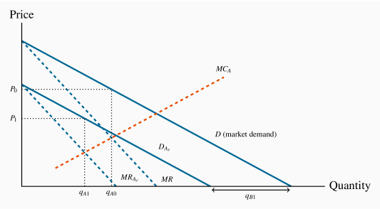
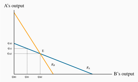
We can develop an optimal strategy with the help of Figure 11.4. D is the market demand, and two firms supply this market. If B supplies a zero output, then A would face the whole demand, and would maximize profit where MC=MR. Let this output be defined by  . We transfer this output combination to Figure 11.5, where the output of each firm is on one of the axes—A on the vertical axis and B on the horizontal. This particular combination of zero output for B and for A is represented on the vertical axis as the point .
Instead, suppose that B produces a quantity  in Figure 11.4. This reduces the demand curve facing A correspondingly from D to
  , which we call A's residual demand. When subject to such a choice by B, firm A maximizes profit by producing where
  , where
  is the marginal revenue corresponding to the residual demand . The optimum for A is now
  , and this pair of outputs is represented by the combination
  in Figure 11.5.
Firm A forms a similar optimal response for every possible output level that B could choose, and these responses define A's reaction function. The reaction function illustrated for A in Figure 11.5 is thus the locus of all optimal response outputs on the part of A. The downward-sloping function makes sense: The more B produces, the smaller is the residual market for A, and therefore the less A will produce.
But A is just one of the players in the game. If B acts in the same optimizing fashion, B too can formulate a series of optimal reactions to A's output choices. The combination of such choices would yield a reaction function for B. This is plotted as  in Figure 11.5.
An equilibrium is defined by the intersection of the two reaction functions, in this case by the point E. At this output level each firm is making an optimal decision, conditional upon the choice of its opponent. Consequently, neither firm has an incentive to change its output; therefore it can be called the Nash equilibrium.
Any other combination of outputs on either reaction function would lead one of the players to change its output choice, and therefore could not constitute an equilibrium. To see this, suppose that B produces an output greater than  ; how will A react? A's reaction function indicates that it should choose a quantity to supply less than
  . If so, how will B respond in turn to that optimal choice? It responds with a quantity read from its reaction function, and this will be less than the amount chosen at the previous stage. By tracing out such a sequence of reactions it is clear that the output of each firm will move to the equilibrium
  .
.
Application Box 11.1 Cournot: Fixed costs and brand
Why do we observe so many industries on the national, and even international, stages with only a handful of firms? For example, Intel produces more than half of the world's computer chips, and AMD produces a significant part of the remainder. Why are there only two major commercial aircraft producers in world aviation – Boeing and Airbus? Why are there only a handful of major North American suppliers in pharmaceuticals, automobile tires, soda pop, internet search engines and wireless telecommunications?
The answer lies primarily in the nature of modern product development. Product development (fixed) costs, coupled with a relatively small marginal cost of production, leads to markets where there is enough space for only a few players. The development cost for a new cell phone, or a new aircraft, or a new computer-operating system may run into billions, while the cost of producing each unit may in fact be constant. The enormous development cost associated with many products explains not only why there may be a small number of firms in the domestic market for the product, but also why the number of firms in some sectors is small worldwide.
The Cournot model yields an outcome that lies between monopoly (or collusion/cartel) and competitive market models. It does not necessarily assume that the firms are identical in terms of their cost structure, although the lower-cost producer will end up with a larger share of the market.
The next question that arises is whether this duopoly market will be sustained as a duopoly, or if entry may take place. In particular, if economic profits accrue to the participants will such profits be competed away by the arrival of new producers, or might there be barriers of either a 'natural' or 'constructed' type that operate against new entrants?