Define the key revenue and profit concepts that neoclassical economists use
Identify the defining characteristics of the neoclassical theory of perfect competition
Explain the two rules of short run profit maximization for perfectly competitive firms
Analyze five possible cases of short run profit maximization under perfect competition
Derive the short run supply curve using the rules of short run profit maximization
Investigate the dynamic adjustment in the case of long run profit maximization
Explore implications and criticisms of the perfectly competitive model
Examine Marx’s theory of profit rate equalization and the related transformation problem
Neoclassical Revenue and Profit Concepts
In chapter 7, we focused almost exclusively on the factors that determine production cost, or the outlays that are required for a firm to obtain inputs for production. To understand the concept of profit, we must also understand something about the monetary receipts from the sale of the firm’s product, also known as total revenue (TR). If a firm only sells a single product then we can write total revenue as we did in chapter 5 where P is the price of the product and Q is the quantity sold. That is:
We need to define two other related revenue concepts. The first is average revenue (AR), which is the revenue per unit of output sold. It is defined as follows:
For example, if a firm’s TR is $5000 and 1000 units of output are produced, then the AR is $5 per unit.
The other concept that we need to define is marginal revenue (MR). Marginal revenue refers to the additional revenue resulting from the sale of an additional unit of output. It is defined as follows:
For example, if a firm’s TR rises by $600 and its output increases by 300 units, then the MR is $2 per unit.
We cannot say anything at this stage about the behavior of TR, AR, and MR because we need more specific information about the characteristics of the marketplace. These concepts are developed at greater length in the next section.
First, however, we must consider what neoclassical economists mean by the term “profit,” which brings together the revenue and cost concepts that we have been discussing. It turns out that accountants define profit very differently from neoclassical economists, and so it is important to contrast the two definitions of profit. Accounting profit refers to the difference between TR and explicit costs. Explicit costs include all out-of-pocket costs or monetary costs, such as the payment of wages, rent, and interest. We can write the definition as follows:
By contrast, neoclassical economists argue that accountants do not account for all the costs of production because some costs are not associated with out-of-pocket, monetary payments. Costs that do not carry with them explicit, monetary payments are called implicit costs. For example, suppose that the owner of the pizzeria is also the cook. Because she is the owner, she does not pay herself a wage (although she hopes to keep any profit that her firm earns). Because her labor is a resource used in production, it could be used elsewhere for some productive activity. That is, the owner could earn a wage or salary elsewhere and so her labor has an opportunity cost. The neoclassical economist, therefore, wishes to include the cost of this labor even though it has no explicit payment associated with it. Similarly, if the owner uses her personal computer to maintain the financial records of the firm, then the cost of this self-owned resource should be included as well even though the business did not directly incur a cost to purchase the computer. Additionally, if the owner invested her own financial capital in the business, then she incurs an opportunity cost in the form of interest and dividend income that would have been earned from other worthy investments. All these implicit costs should be included in any profit calculation, according to neoclassical economists. Neoclassical economists, therefore, define economic profit in the following way:
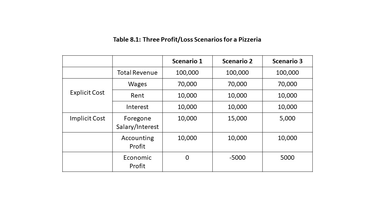
Let’s consider an example in which the pizzeria earns $100,000 in revenue in one month. Table 8.1 contains three scenarios. All numerical values are in dollar terms.
In each scenario the explicit costs are the same and only the implicit costs differ. Because the explicit costs are the same in all three scenarios, the firm earns $10,000 in accounting profit in all three cases. Because the implicit costs differ, however, the economic profit is different in each of the scenarios. Despite the positive accounting profit of $10,000 in Scenario 1, the economic profit is $0 due to the implicit cost of $10,000. An economic profit of zero might appear to be an unpleasant situation for the firm, but in fact it is the opposite. The firm is earning enough revenue to cover its explicit costs and the foregone salary and interest of the owner. That is, the owner could not earn more in any other line of business. It is said that the firm enjoys a normal profit equal to $10,000 in this case.
In Scenario 2, the economic profit is -$5,000. That is, the revenue the firm earns is not sufficient to cover both the explicit and implicit costs. Even though the firm earns a profit on paper (i.e., a positive accounting profit), in a real sense, the firm is losing money. If the owner shut down the business and took her next best opportunity, she would earn an additional $5,000. As a result, the firm earns less than a normal profit in this case.
In Scenario 3, the economic profit is $5,000. The firm earns enough revenue to more than cover all explicit and implicit costs. In this case, if the owner shut down the business to produce elsewhere, she would actually lose $5,000. The firm clearly earns more than a normal profit in this industry. It should now be clear why neoclassical economists focus exclusively on economic profit. Economic profit is ultimately what affects a firm’s decision to remain in an industry or to leave an industry. Since accounting profit is the same in all three scenarios, it is not a proper guide to managerial decision making.
Although it was not mentioned in Chapter 7, all the cost curves that we discussed in the last chapter include both explicit and implicit production costs. Unless otherwise noted, any reference to production cost in neoclassical theory should be understood to include both kinds of cost because those are the costs that influence firm behavior according to neoclassical economists.
The Concept of Market Structure and the Meaning of Perfect Competition
We now wish to take a closer look at how the revenue measures defined in the last section behave as output changes. To accomplish this task, we must first discuss the concept of market structure. Market structure refers to all the characteristics of the marketplace that shape and influence how firms interact with their customers and with their competitors. Three key dimensions are used to distinguish between the different types of market structure:
The number and size of sellers
The ease of market entry and exit
The degree of product differentiation
How these characteristics combine in a specific market determines the degree of market power that each firm has in that market. Market power refers to the ability of a firm to raise the price of its product without losing all of its sales. A firm’s market power is greater when the reduction in quantity demanded is smaller for a given increase in price. For example, Figure 8.1 shows two demand curves facing two different firms in two different markets for a similar good.
The firm facing a flatter demand curve possesses less market power because the rise in price from P1 to P2 leads to a much sharper reduction in quantity demanded. The firm facing a steeper demand curve possesses considerable market power.Figure 8.2 represents the market power spectrum.
Each of these market structures is distinguished along the lines of the three dimensions mentioned previously. The only market structure that we will examine in this chapter is perfect competition. According to neoclassical economists, a perfectly competitive market structure has the following three characteristics:
A large number of sellers and buyers
No barriers restrict the freedom of buyers or sellers to enter or exit the market
Each firm produces a homogeneous or standardized product
We should consider a few examples of actual markets that closely resemble perfectly competitive markets. For example, agricultural markets are highly competitive. The markets for wheat or corn have many buyers and sellers, and these crops are found to be very similar when we compare the product of one seller with that of another. It is also relatively easy for buyers and sellers to enter and exit these markets. Other examples include the markets for precious metals (e.g., gold and silver) and markets for corporate stock. In these markets, the standardization of the thing being sold is plainly seen.
The implication is that no seller or buyer in a perfectly competitive market has any market power. That is, each seller (or buyer) is a price-taker, and so is powerless to change the market price. In all these markets, competition is so intense that no single buyer or seller has the power to raise or lower her price above or below the market price without reducing her sales to nothing (in the case of a price increase) or needlessly sacrificing revenue (in the case of a price decrease). The graphical analysis of a price-taking firm is taken up in the next section.
Neoclassical economists assert that the phrase “perfect competition” is entirely descriptive in nature. Indeed, these three characteristics appear to simply describe certain features of specific markets. It should be noted, however, that the perfectly competitive market structure is the normative standard in neoclassical economics as well. That is, it is the moral ideal toward which market capitalist economies should strive, according to this school of thought. The reason neoclassical economists are such strong advocates of perfect competition is that such markets can be shown to lead to economic efficiency, as defined in chapter 2. Later in this chapter, we will see how neoclassical economists arrive at this result.
The Revenue Structure of a Perfectly Competitive Firm
In order to determine a perfectly competitive firm’s revenue pattern, we must first analyze the demand curve facing such a firm. From Chapter 3, we know that the market demand curve is downward sloping due to the law of demand, but the demand curve facing the individual firm is horizontal, as shown in Figure 8.3.
The reason for the difference is that the individual perfectly competitive firm is a price-taker and only faces a tiny segment (d) of the entire market demand (D). If the perfectly competitive firm attempts to raise the price above P1, then the quantity demanded (q) will fall to 0 units because every buyer can obtain a perfect substitute from a competitor at a price of P1. Additionally, it makes no sense for the firm to reduce the price below P1 because the firm can sell as much as it wants at the market price. It will sacrifice revenue needlessly if it cuts price because a price cut is not necessary to sell additional units. The firm is so small relative to the entire market that plenty of customers exist at the market price. We can also state that demand is infinitely elastic in the case of the demand curve facing the perfectly competitive firm. The smallest price increase will cause quantity demanded to fall to zero, and the smallest price cut will cause quantity demanded to soar.Figure 8.4 shows the TR curve for a perfectly competitive firm that faces a constant market price of $3 per unit.
The graph on the left in Figure 8.4 shows that the area of the box under the demand curve is equal to total revenue since it is calculated as the product of price and quantity demanded. Furthermore, an additional unit can be sold at a price of $3 because the firm is a price-taker. The graph on the right shows what happens to total revenue as the quantity sold rises. It increases in a linear fashion because with each additional unit sold, the TR rises by the amount of the price of that unit, which is constant since the firm is a price-taker. Hence, the 101st unit raises TR from $300 to $303.
We can also see that the TR curve is linear because TR = Pq, and the price is constant. Hence, the TR curve will have a zero intercept and a constant slope. If the price rises, then the TR curve will still rise from the origin, but the line will become steeper. That is, TR will rise more quickly as quantity rises. On the other hand, if the price decreases, then the TR curve will become flatter, indicating that TR rises more slowly. In addition, a price increase will shift the demand curve facing the firm upwards, and a price reduction will shift the demand curve facing the firm downwards.
Next, we wish to investigate the behavior of marginal revenue as the quantity sold changes. In the case of a price-taking firm, a unit increase in quantity always increases TR by the amount of the price. Hence, the MR is always equal to the price in the case of a perfectly competitive firm. That is:
In Figure 8.4, for example, the MR of the 101st unit is $3 per unit. Also, the slope of the TR curve is equal to the constant price, which in turn is equal to ∆TR/∆q. Hence, mathematically, we can see that MR = P. The MR curve is, therefore, the same as the horizontal demand curve facing the firm.
We can also consider the behavior of average revenue as the price changes. The AR in the case of a perfectly competitive firm is equal to the price as shown below:
In Figure 8.4, for example, the AR when 100 units are sold is equal to $300/100 units or $3 per unit. Similarly, the AR when 101 units are sold is equal to $303/101 units or $3 per unit. Since AR = P, the AR curve is also the same as the horizontal demand curve facing the perfectly competitive firm. Figure 8.5 shows the MR and AR curves on a graph.
All the revenue measures can also be expressed in tabular form as shown in Table 8.2.
Methods of Profit Maximization in the Short Run
The behavioral assumption that neoclassical economists impose is that all firms seek to maximize economic profit. A considerable amount of disagreement exists as to whether profit maximization is the primary objective of firms. Some critics argue that managers of modern corporations pursue revenue growth and market share much more aggressively than maximum profits. Others argue that firms consider their broader sense of social responsibility, which includes a commitment to the firm’s stakeholders (e.g., customers, the community, employees) rather than simply a commitment to the firm’s shareholders. Finally, it might be argued that firms balance multiple and competing objectives in their operations and that no single goal should be elevated above the others. Whatever may be the case, we will assume that the firm strives only to maximize its economic profit, in accordance with the neoclassical theory of the firm.
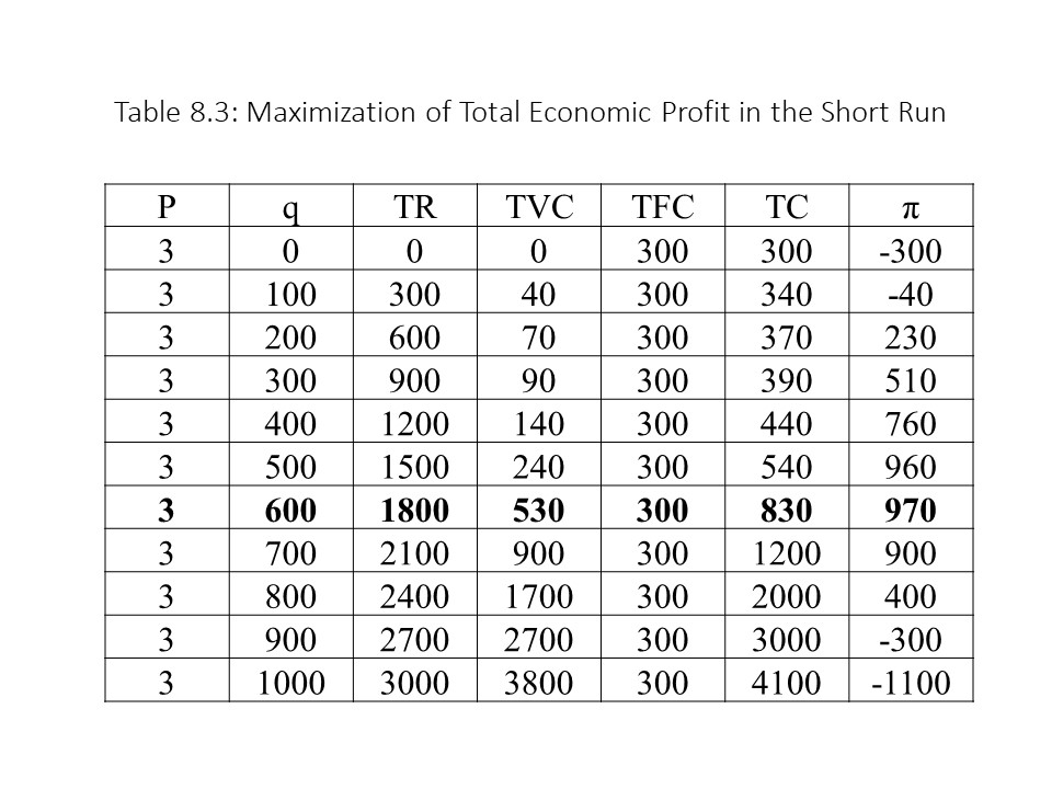
Because the perfectly competitive firm takes the market price as given, it need not ask which price is the best price to charge. In the short run, the only decision the firm must make is how much output to produce to maximize its economic profit. One way for the firm to achieve this goal is to compare TR and TC at each output level. Because the difference is the total economic profit (π), the firm can simply select the output level that maximizes that difference. Table 8.3 provides an example of a firm that aims to solve this profit maximization problem in the short run.
According to Table 8.3, the firm will maximize its economic profit by producing 600 units of output. At that output level, its economic profit will be $970. One can also see that if the firm produces too little or too much, then it will experience economic losses. Producing too little means that the firm fails to take sufficient advantage of labor specialization and the division of labor. Producing too much means that the firm fails to recognize the negative impact that diminishing returns to labor carries for profitability.Figure 8.6 shows two ways of graphically representing the maximum economic profit.
Figure 8.6 shows that economic losses exist to the left of the first break-even point because TC exceeds TR. At the break-even point, TC = TR and so economic profit is $0. Earlier in the chapter, it was argued that an economic profit of zero is still acceptable to the firm because all costs are covered. Because the opportunity costs are covered as well, the firm earns a normal profit. In between the two break-even points, the firm’s revenues exceed its costs. Therefore, positive economic profits are earned over that range of output. At a single output level, however, the gap between the TR and the TC is maximized. At that point where Q = 600 units, the economic profit is at a maximum.
The graph on the right represents the economic profit curve. It measures the difference between the TR and the TC, as shown in the graph on the left. The break-even points occur where the economic profit curve crosses the horizontal axis. Clearly, it reaches its maximum where Q = 600 units.
A second way to determine the profit-maximizing approach is less obvious but more useful. Managers generally do not have access to information about TR and TC at every possible output level. Instead, they base their production decisions on how profits rise or fall with small adjustments to output. This information is contained in the MC and MR measures, which have been calculated and are shown in Table 8.4.
As Table 8.4 shows, MR is constant and equal to the product price of $3 per unit. The MC, on the other hand, falls and then rises for reasons already explained in chapter 7. We might start by asking whether the firm would find it profitable to produce the 100th unit of output. Since the sale of that additional unit will generate $3 of additional revenue and its production will add only $0.40 to cost, that unit will clearly add to the firm’s economic profit. The 200th unit will also add to the firm’s economic profit because the MR of $3 per unit clearly exceeds the MC of $0.30 per unit. In fact, the firm will continue to increase its output as long as MR exceeds MC. Once the firm reaches the 600th unit, the MR of $3 just barely exceeds the MC of $2.90 per unit and so it will be produced. If the firm increases its output any further, however, the MC of $3.70 will exceed the MR of $3 per unit and so it will not be profitable to produce that unit. The firm should, therefore, stop production at 600 units.
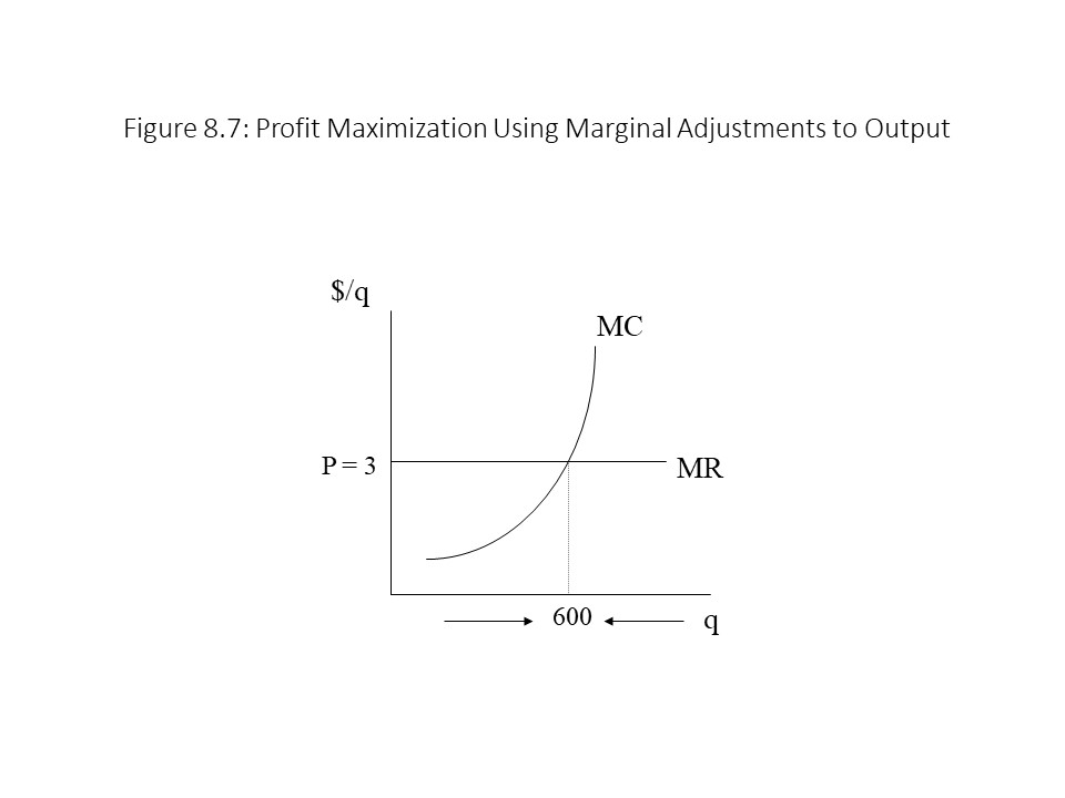
Even though MR and MC are not exactly equal at 600 units, they are close to equal. If we were to show more data, we could imagine increasing the output level somewhat above 600 units (but not as high as 700 units) until we reach the point where MR exactly equals MC. We know that MC will continue to rise due to diminishing returns to labor. The law of diminishing returns is the reason that the firm ceases production at a specific level of output in the short run. Beyond a certain point, the upward pressure on unit cost simply becomes too great. Figure 8.7 provides a graphical representation of how marginal adjustments to output can be used to determine the profit maximizing level of output for a perfectly competitive firm in the short run.
We can summarize how these marginal adjustments lead to the profit-maximizing choice of output:
If MR > MC, then the firm should increase its output.
If MR < MC, then the firm should reduce its output.
If MR = MC, then the firm should neither increase nor decrease its output.
It should also be noted that P = MR in the case of the perfectly competitive firm. Therefore, the rule that MR = MC can be written as P = MC for the perfectly competitive firm. Indeed, this condition is the first rule of profit maximization when we use the marginal approach.
Although the first rule of profit maximization is a necessary condition to ensure that profits are maximized in the short run, it is not a sufficient condition. That is, some instances arise in which a perfectly competitive firm would earn a greater profit by shutting down and producing zero units of output than by producing at the output level at which P = MC.
When would the firm decide to shut down? The second rule of profit maximization states that a firm will shut down when the product price falls below the firm’s average variable cost (AVC). Another way of stating this rule is to state that the firm will only produce at the output level where MR = MC when the product price is at least as great as AVC. That is, the firm will only produce when P ≥ AVC. This rule might seem entirely arbitrary to the reader, but it can be proven with the help of a little basic algebra.
As we have seen, if the firm operates then its profits from operating (πo) are the following:
On the other hand, if the firm shuts down then its profits from shutting down (πSD) are also:
We can say more about the profits from shutting down. If the firm produces no output, then its revenues are zero. Furthermore, its variable costs are $0 because the firm will not purchase any labor. Hence, the profits from shutting down may be written as:
We can now compare the firm’s profits from operating with the firm’s profits from shutting down. In fact, the firm will only operate if the profits from operating are at least as great as the profits from shutting down. That is, the firm should operate if and only if πo ≥ πSD. We can now derive the second rule of profit maximization as follows:
What this condition means is that the firm must earn enough revenue to cover its variable costs. If it does not earn this much revenue, then it makes more sense for the firm to shut down. Shutting down will cause the firm to lose its revenue, but firing all the workers will also allow the firm to eliminate its variable costs. The firm’s loss will then be reduced to its TFC.
Five Possible Cases of Short Run Profit Maximization
Given the marginal approach to short run profit maximization, we can identify five possible cases that might arise depending on the magnitude of the product price. Each of these cases as well as their implications for profitability are as follows:
In each of the five cases, we will consider how the two rules of short run profit maximization influence the graphical analysis of the situation. Again, the firm should 1) produce where MR = MC conditional upon 2) P ≥ AVC. Otherwise, the firm should shut down and produce zero units of output.
Case 1 is the case of a positive economic profit as shown in Figure 8.8.
We begin our analysis of this case by finding the point at which MR = MC. Moving straight down from the intersection of these two curves to the horizontal axis gives us an output level of 100 units. Before we declare this output level to be the profit-maximizing choice, we need to check whether P ≥ AVC. In this case, it is greater. Even though the specific AVC has not been identified in the graph, we know that P exceeds AVC because at q* the MR curve is higher than the AVC curve. Therefore, the profit-maximizing output level is 100 units.Figure 8.8 to calculate TR, TC, and π. For example, TR is calculated as Pq so in this case TR is equal to $100 (= $1.00 per unit times 100 units). The TC is calculated as the product of ATC and q. To understand the reason, just recall that ATC = TC/q. Therefore, TC may be written as ATC·q. In this case, TC is equal to $80 (= $0.80 per unit times 100 units). We can now determine the total economic profit as the difference between TR and TC. In this case, π = $20 (= $100 – $80) and is simply the area of the shaded region in the graph.
Case 2 is the case of an economic profit of zero as shown in Figure 8.9.
Again, we find the intersection of MR and MC to occur at 100 units of output. In addition, at that output level, the MR curve lies above the AVC curve and so the firm will operate. The profit-maximizing output level is 100 units as before. The TR in this case is $100 (= $1.00 per unit times 100 units). Because the ATC is also $1.00 per unit, the TC in this case is $100 as well. As a result, the economic profit is zero. Another way to see why economic profit is equal to zero is to notice that the box representing TR in the graph also represents TC. The reader should recall that the firm earns a normal profit in this case, and so this situation is not unacceptable to the firm. That is, the firm could not earn a greater profit in any other industry.Figure 8.10.
That is, shutting down is an even worse option. Let’s see why. The intersection of MR and MC occurs at 100 units of output as before and P = $0.80 is clearly above AVC = $0.60 at that output level. Hence, the firm will operate. The firm’s TR is equal to $80 (= $0.80 per unit times 100 units) and the firm’s TC is equal to $100 (= $1.00 per unit times 100 units). The firm’s economic profit is, therefore, equal to -$20 (= $80 minus $100). This loss is represented in Figure 8.10 as the top shaded box.
Why would the firm operate in this situation in the short run? If the firm shuts down, we know that its economic profit is always equal to – TFC. We can show the TFC graphically as the product of AFC and q. The reason is that AFC = TFC/q. Therefore, TFC = AFC·q. Furthermore, since ATC = AFC+AVC, the AFC = ATC – AVC. Hence, we can calculate the AFC in this case to be $0.40 per unit (= $1.00 per unit – $0.60 per unit), and the TFC is then equal to $40 (= $0.40 per unit times 100 units). Therefore, the economic profit from shutting down (= – TFC) is -$40. Clearly, this loss is much greater than the loss from operating. The loss from shutting down is equal to the two shaded areas combined. It follows that the firm will operate to maximize its economic profit. Certainly, the two rules of profit maximization led us to this conclusion much more quickly!
Case 4 is the case of a firm that is indifferent between operating and shutting down because its profit/loss situation is the same in either case. Figure 8.11 represents this case.
In this case, the intersection between MR and MC occurs at 100 units of output as before. The price, however, is exactly equal to AVC at this output level. The second rule of profit maximization requires that price be greater than or equal to AVC for the firm to operate. This condition is fulfilled and so the firm will operate. We can also see that TR is equal to $80 (= $0.80 per unit times 100 units) and TC is equal to $100 (= $1.00 per unit times 100 units). The firm’s economic profit is, therefore, equal to -$20 (= $80 – $100). In addition, because the AFC = $0.20 per unit, the TFC = $20 (= $0.20 per unit times 100 units). If the firm shuts down then, its economic profit will be equal to -$20 (= –TFC). Clearly, the profit from operating is the same as the profit from shutting down. Because the firm is indifferent between operating and shutting down, by convention, we conclude that the firm will operate.
Students of economics are often puzzled by the conventional conclusion that a firm operates even though its economic profit is the same whether it operates or shuts down. In other words, why doesn’t the owner just stay in bed if the profit/loss situation is the same either way? Although it may seem strange, the reader should remember that the revenue is sufficient to cover all costs, including the opportunity cost of operating the firm, which might include the value the owner places on additional sleep!
Case 5 is the only case in which the firm decides to shut down and produce zero units of output as shown in Figure 8.12.
Again, the MR = MC intersection occurs at 100 units of output, but this time, the price of $0.70 per unit is below the AVC of $0.80 per unit. The second rule of profit maximization indicates that the firm should shut down in this case. The economic profit in this case is equal to –TFC. Because the AFC is $0.20 per unit, the TFC equals $20 (= $0.20 per unit times 100 units). The economic profit is, therefore, -$20. The careful reader might wonder how we can calculate TFC at an output level of 100 units when the firm has opted to produce zero units. The reason is that TFC is the same at all output levels so if we determine the TFC at 100 units of output, we also know the TFC at zero units of output.
It should also be noticed that if the firm had operated at 100 units of output, then its TR would equal $70 (= $0.70 per unit times 100 units) and its TC would equal $100 (= $1.00 per unit times 100 units). Its economic profit would then be -$30. That is, its economic loss from operating would exceed its economic loss from shutting down. In the graph, the economic loss from operating is equal to the sum of the two shaded regions. Only the top shaded region (equal to the TFC) is lost if the firm shuts down.
The Derivation of the Short Run Supply Curve
Now that we have shown how the perfectly competitive firm maximizes its economic profit in the short run, we can use the analysis to derive the firm’s short run output supply curve. Figure 8.13 shows a series of MR curves corresponding to different prices as determined in the competitive market for this product.
As the market price falls, the MR curve shifts downward. At the highest price of P4, the two rules of profit maximization indicate that q4 should be produced. At that output level, MR = MC and P > AVC. When the price declines to P3, the firm will produce q3, and the break-even point will be reached since P = ATC. When the price declines further to P2, q2 is produced and the shutdown point is reached since P = AVC. Finally, when the price falls to P1, the firm maximizes its economic profit by shutting down and producing zero units of output because P < AVC. This analysis has allowed us to observe the different quantities of output supplied at different market prices, other factors held constant. In other words, the short run analysis of profit maximization has made possible the derivation of the firm’s output supply curve. Because the intersections of MR with MC determine the profit-maximizing output levels, we can conclude that the supply curve is the MC curve above the minimum AVC. In Figure 8.13, the supply curve is the darkened portion of the MC curve plus the vertical axis below the minimum AVC because the firm produces zero units of output when the market price falls below that level.Figure 8.14 shows the perfectly competitive firm’s short run supply curve without the interference of the unit cost and MR curves.This analysis reveals the reason why we drew the supply curves in chapter 3 as suspended without a vertical intercept. We can also reinterpret the market supply curve. In chapter 3, it was explained that the market supply curve is the aggregation of many individual sellers’ supply curves, which we can obtain through horizontal summation. We now see that the market supply curve is also the horizontal summation of the individual firms’ MC curves.Figure 8.15 than we previously had.
Long Run Profit Maximization
We now turn to an analysis of profit maximization in the long run when all inputs are variable. Because capital inputs are not fixed in the long run, firms will enter the industry if economic profits exist, and they will exit the industry if economic losses exist. For the purposes of this analysis, we will assume that all firms possess identical short run ATC curves. This assumption is reasonable so long as all firms have access to the same production technologies and face the same opportunity costs. At this stage, we will ignore the adjustments that firms make to their plant sizes and focus exclusively on the impact that the entry and exit of competing firms has on the profit/loss situations of firms in the industry.
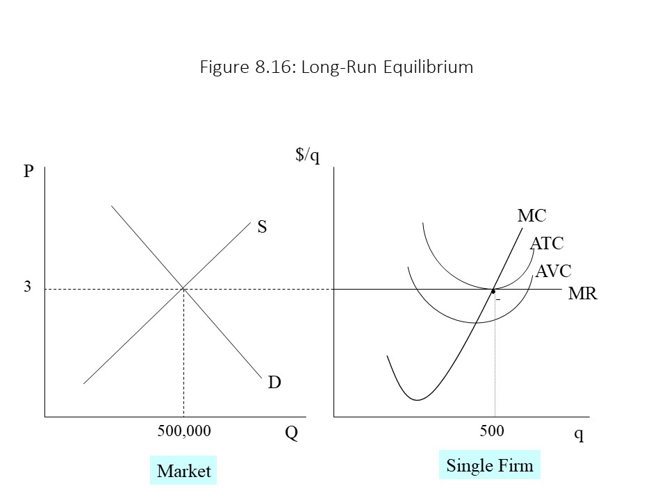
It turns out that the long run equilibrium outcome for a firm in a perfectly competitive market is the break-even case we considered in our analysis of the short run. That is, the market price is determined competitively through the interaction of supply and demand, and each firm earns an economic profit of zero as shown in Figure 8.16.
Why does this case represent the long run equilibrium outcome? The reason is that short run deviations from this situation produce an inherent long run tendency to change in the direction of this outcome. For example, in Figure 8.17, the market price and quantity exchanged begin at P1 and Q1, and the firm produces q1 units of output.
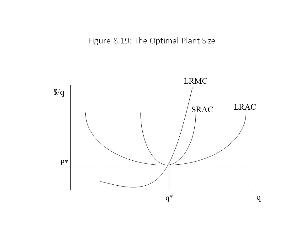
Now assume that a short run increase in demand causes the demand curve to shift to D2. The increase in the market price to P2 causes the firm’s MR curve to shift upwards from MR1 to MR2. The firm’s profit-maximizing choice of output, therefore, rises from q1 to q2. The price charged now exceeds ATC resulting in positive economic profits. In the long run, firms outside the industry respond to the resulting economic profits, which function as a signal that they should enter this industry. As the number of sellers in the industry increases, the market supply curve shifts rightward from S1 to S2. The market price falls to P3, and the economic profits return to zero as the firm reduces output to the original level of q1. It should be noted that the market price returns to its original level, but the market quantity exchanged has increased from Q1 to Q3. This result is argued to be consistent with Adam Smith’s Invisible Hand in that the free market has reallocated a part of society’s resources toward the production of this product for which consumer demand has grown.Figure 8.18.The decrease in the market price to P2 causes the firm’s MR curve to shift downwards from MR1 to MR2. The firm’s profit-maximizing choice of output, therefore, falls from q1 to q2. The price charged is now below ATC resulting in economic losses. In the long run, firms inside the industry respond to the economic losses, which function as a signal that they should exit this industry. As the number of sellers in the industry decreases, the market supply curve shifts leftward from S1 to S2. The market price rises to P3, and the economic profits return to zero as the firm increases output to the original level of q1. It should be noted that the market price returns to its original level, but the market quantity exchanged has decreased from Q1 to Q3. This result is also argued to be consistent with Adam Smith’s Invisible Hand in that the free market has reallocated a part of society’s resources away from the production of this product for which consumer demand has fallen.Figure 8.19.
This result is expected because, as we have seen, whenever a marginal contribution is below an average, the average falls and whenever the marginal contribution is above an average, the average rises.
The firm will maximize long run economic profits by equating P and LRMC. Now suppose that the profit-maximizing choice is such that price exceeds LRATC. Then economic profits are made and firms will enter, driving the price down. As the price falls, the firm will reduce its plant size. Alternatively, suppose the profit-maximizing choice is such that the price is below LRATC. Then economic losses exist, and firms will exit the industry pushing the price up. As the market price rises, the firm will increase its plant size. Eventually, the firm will produce at output level q* where the market price is equal to LRMC and LRATC. In that situation, the firm is breaking even in the long run. It should also be noted that the plant size that corresponds to this output level allows the firm to produce at minimum SRATC and minimum LRATC. That is, the firm exhausts the gains from specialization and the division of labor in this plant but does not increase production so much that diminishing returns to labor begin to drive up per unit cost. Furthermore, it exhausts the gains from economies of scale but does not enter the region of diseconomies of scale. It is the optimal plant size for this reason.
The Derivation of the Long Run Industry Supply Curve
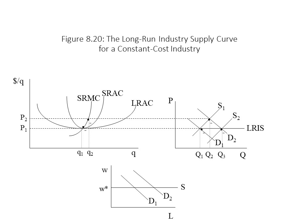
We can use our analysis of long run profit maximization to derive the long run industry supply (LRIS) curve.[2] The LRIS curve may possess different shapes depending on the way in which input prices respond as additional firms enter the market. If an abundance of the necessary inputs exists, then input prices might remain constant as additional firms enter the market. This type of industry is referred to as a constant-cost industry. Figure 8.20 shows how long run profit maximization may be used to derive the LRIS curve in a constant-cost industry.
In Figure 8.20, a short run increase in demand from D1 to D2 causes an increase in the product price from P1 to P2. As a result, the firm expands its output in the short run from q1 to q2. The resulting economic profits cause competitors to enter the industry. As additional firms enter, they increase the demand for inputs, such as labor, but because input supplies are perfectly elastic (i.e., horizontal), input prices (e.g., wages) do not rise. As a result, the LRAC remains fixed. Market supply, therefore, increases from S1 to S2 until the price returns to its original level, and economic profits are again zero. Finally, we can connect the original equilibrium P1 and Q1 with the new equilibrium at P1 and Q3 with a straight line. This horizontal line is the LRIS curve for a constant-cost industry. It shows that the market can expand in the long run without any upward pressure on the product price, precisely because no upward pressure on the inputs prices occurs with the expansion.
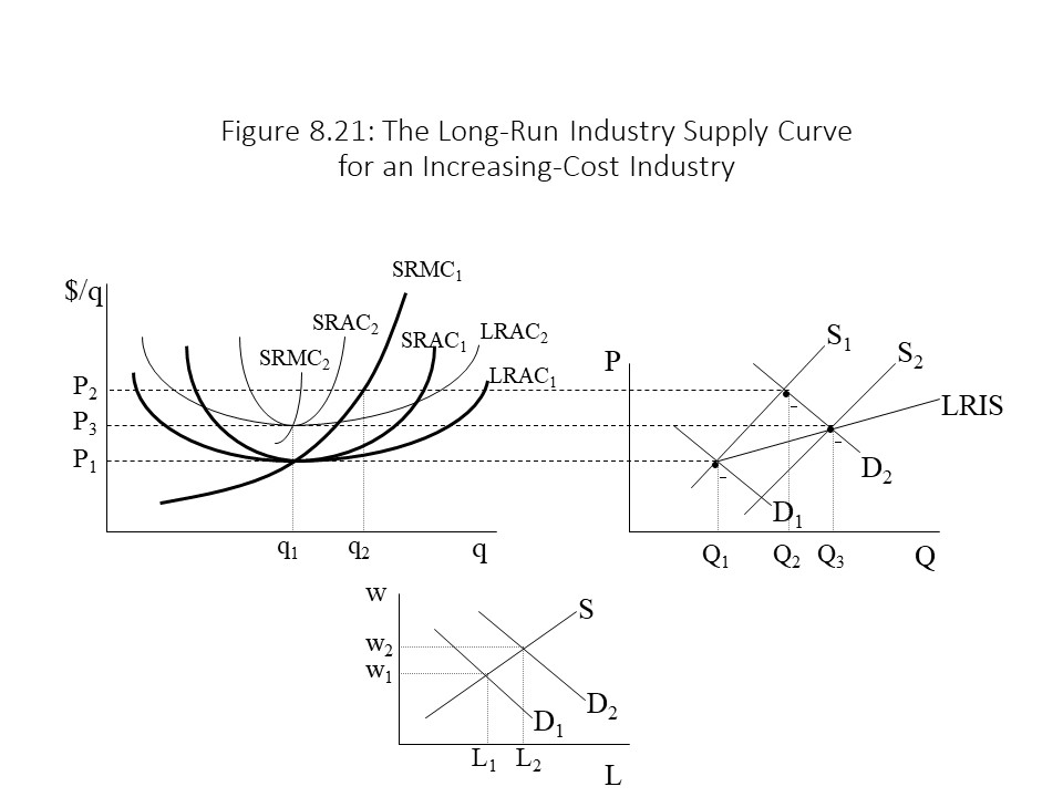
If the necessary inputs are relatively scarce, then input prices are more likely to rise as additional firms enter the market. This type of industry is referred to as an increasing-cost industry. Figure 8.21 shows how long run profit maximization may be used to derive the LRIS curve in an increasing-cost industry.
In Figure 8.21, a short run increase in demand from D1 to D2 causes an increase in the product price from P1 to P2. As a result, the firm expands its output in the short run from q1 to q2. The resulting economic profits cause competitors to enter the industry. As additional firms enter, they increase the demand for inputs, such as labor, and because input supply curves are upward sloping, input prices (e.g., wages) rise. As a result, the LRAC shifts upward due to the rise in unit costs. Market supply, therefore, increases from S1 to S2 until the price declines to P3, at which point economic profits are again zero. Finally, we can connect the original equilibrium P1 and Q1 with the new equilibrium at P3 and Q3 with a straight line. This upward sloping line is the LRIS curve for an increasing-cost industry. It shows that the market can expand in the long run only by putting upward pressure on the product price because upward pressure on the input prices occurs during the expansion.
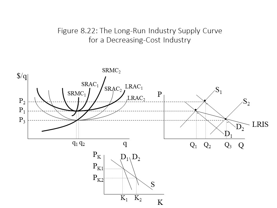
If significant economies of scale exist in the input markets, then input prices may decline as additional firms enter the market. This type of industry is referred to as a decreasing-cost industry. Figure 8.22 shows how long run profit maximization may be used to derive the LRIS curve in a decreasing-cost industry.
In Figure 8.22, a short run increase in demand from D1 to D2 causes an increase in the product price from P1 to P2. As a result, the firm expands its output in the short run from q1 to q2. The resulting economic profits cause competitors to enter the industry. As additional firms enter, they increase the demand for inputs, such as capital, but because input supply curves are downward sloping (reflecting scale economies), input prices (e.g., prices of capital goods) fall. As a result, the LRAC shifts downward due to the reduction in unit costs. Market supply, therefore, increases from S1 to S2 until the price declines to P3, at which point economic profits are again zero. Finally, we can connect the original equilibrium P1 and Q1 with the new equilibrium at P3 and Q3 with a straight line. This downward sloping line is the LRIS curve for a decreasing-cost industry. It shows that the market can expand in the long run even as the product price falls because downward pressure on the input prices occurs during the expansion. This situation has occurred, for example, in the market for desktop and laptop computers due to effective utilization of economies of scale in the production of computer components as the market for computers has grown.
Implications and Criticisms of the Neoclassical Model of Perfect Competition
The major implication of the neoclassical model of perfect competition is that this market structure achieves economic efficiency. In chapter 3, it was explained that competitive market equilibrium leads to the full employment of scarce resources and allocative efficiency. That is, all resources are fully employed and marginal benefit equals marginal cost for each good produced when all markets clear. In that discussion, it was explained that the demonstration of least cost production would be postponed until this chapter. We can now see that long run equilibrium in a perfectly competitive market will lead to least-cost production. The long run equilibrium outcome leads to a price that is just equal to minimum long run average total cost. Hence, productive efficiency is achieved. Because full employment, least-cost production, and allocative efficiency are all achieved in a perfectly competitive market economy, neoclassical economists conclude that this market structure achieves economic efficiency. It is, therefore, the normative standard in neoclassical economics.
Nevertheless, we need to reflect on several major criticisms of the neoclassical model of perfect competition and its efficiency conclusion. First, market demand reflects willingness and ability to pay for the good or service. An individual may desperately need a specific good (e.g., a medication) but at the same time, she cannot afford to purchase the good at the equilibrium price. Because she is at a point on the demand curve that is below the equilibrium price, she will remain in need even when the market clears. To call the outcome an efficient one suggests that it is the most desirable outcome, but it ignores the possibility that many in need will not be able to obtain the product. The reader should recall that neoclassical economists do not distinguish between wants and needs. This criticism of the model is, therefore, a criticism that only heterodox economists emphasize.
A second major criticism of the neoclassical model of perfect competition is that social welfare is defined entirely in terms of the efficient use of resources to satisfy consumer wants. The level of satisfaction derived from productive work is completely ignored. For example, workers may be efficiently employed, but what if they are working 14-hour days over hot stoves or in dangerous coal mines and hate their jobs? Their satisfaction from living in such a society is diminished regardless of how much satisfaction they may derive from consuming material goods. Many workers may prefer to reduce their working hours even if it means reducing their material consumption, but in capitalist economies that choice may not exist. For many workers, the choice is to work long hours or not work at all. Even if part-time work is available, it typically is offered at low pay and without key benefits such as health insurance.
A final criticism of the neoclassical model of perfect competition is that it ignores power relationships. Conflicts between social classes are not possible in the model, which only acknowledges individuals interacting voluntarily in the free market. The notion that the relationship between employer and employee is conflict-ridden is entirely absent. All resource owners compete on the same level. The owners of capital and the owners of labor confront one another as equals in the perfectly competitive marketplace. All take market prices as given and differences in relative power simply do not exist. As we will see in the next section, the Marxian analysis of intensely competitive markets disagrees sharply with these conclusions.
The Marxian Theory of Competitive Profit Rate Equalization
Our purpose in this section is to consider how Marxian economists think about intensely competitive market capitalist economies. As we saw in Chapter 4, Marxian economists place primary emphasis on class conflict in their analyses of capitalism. To understand how this feature of capitalism is emphasized in their analysis of capitalist competition, we must first introduce a new concept that Marxian economists call the organic composition of capital(OCC). The organic composition of capital refers to the degree of constant capital intensity present in a capitalist production process. That is, a capitalist production process that uses relatively more constant capital than variable capital has a higher organic composition of capital than another capitalist production process that uses relatively less constant capital compared with variable capital. To make this definition more precise, we can define the OCC as follows:
According to this definition, the OCC tells us the fraction of the total capital advanced that consists of constant capital. If the total capital advanced is $1000 and the constant capital advanced is $700, then the OCC is 70%. In the extreme case that no constant capital is advanced (c = 0), the OCC equals 0. On the other extreme, if the entire capital consists of constant capital (v = 0), then the OCC equals 1 or 100%.
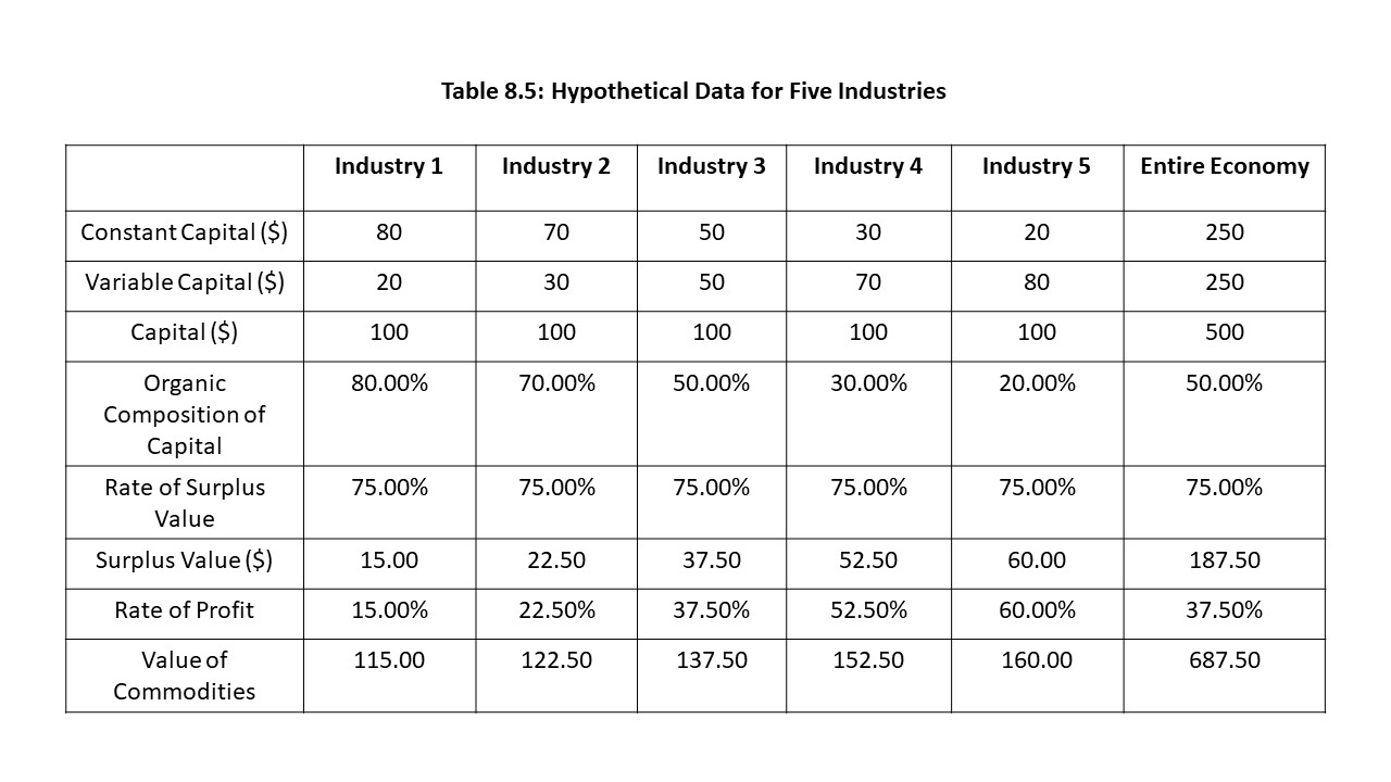
We are now able to consider a simple example of a capitalist economy with only five industries. Table 8.5 contains hypothetical data for the five industries.
In this example, each of the firms advances $100 worth of capital, but the organic compositions of capital are very different. Industry 1 has a very high OCC of 80% whereas Industry 5 has the lowest OCC of only 20%. In neoclassical terminology, Industry 1 is very “capital-intensive” and Industry 5 is very “labor-intensive.” The rates of surplus value are also assumed to be the same across the industries. Specifically, the rate of surplus value (s/v) is assumed to equal 75% in each industry.[3]
These assumptions of different OCCs and uniform rates of surplus value lead to differences in the rates of profit across the sectors. Why? Recall that labor-power is the only commodity that creates new value (and thus surplus value) in the Marxian framework. When an industry uses relatively more variable capital, it will necessarily produce more surplus value (assuming the same degree of exploitation or rate of surplus value) across industries. That is the reason that Industry 5 produces the most surplus value and has the highest rate of profit. Similarly, it is the reason that Industry 1 produces the least surplus value and has the lowest rate of profit. As the reader can see by looking at what happens to the OCC and the rates of profit from Industries 1 through 5, as the OCC falls, the rate of profit rises.
Because capitalists measure the profitability of their activities using the rate of profit, this situation is highly unstable in a competitive capitalist economy. Think about it. Why would a capitalist want to invest $100 in Industry 1 and earn a 15% return when she can invest the same $100 in Industry 5 and earn a 60% return. Capital’s search for the highest rate of profit should cause it to exit industries that have low profit rates due to high OCCs and to enter industries that have high profit rates due to low OCCs.
In everyday life, we do not observe profit rates that are much higher in industries that use relatively more variable capital (e.g., garment-making) and profit rates that are much lower in industries that use relatively more constant capital (e.g., the automobile industry). The problem we face then is to explain how the rates of profit equalize across industries so that the same amount of capital generates approximately the same return regardless of where it is invested. From a static perspective, the solution to this problem requires that we calculate the general rate of profit (r) for this capitalist economy. The general rate of profit that applies to all capital once the profit rates have equalized may be calculated by dividing the aggregate surplus value (S) for the entire economy by the aggregate capital advanced (C+V) for the entire economy. We can calculate the general rate of profit in this example in the following way:
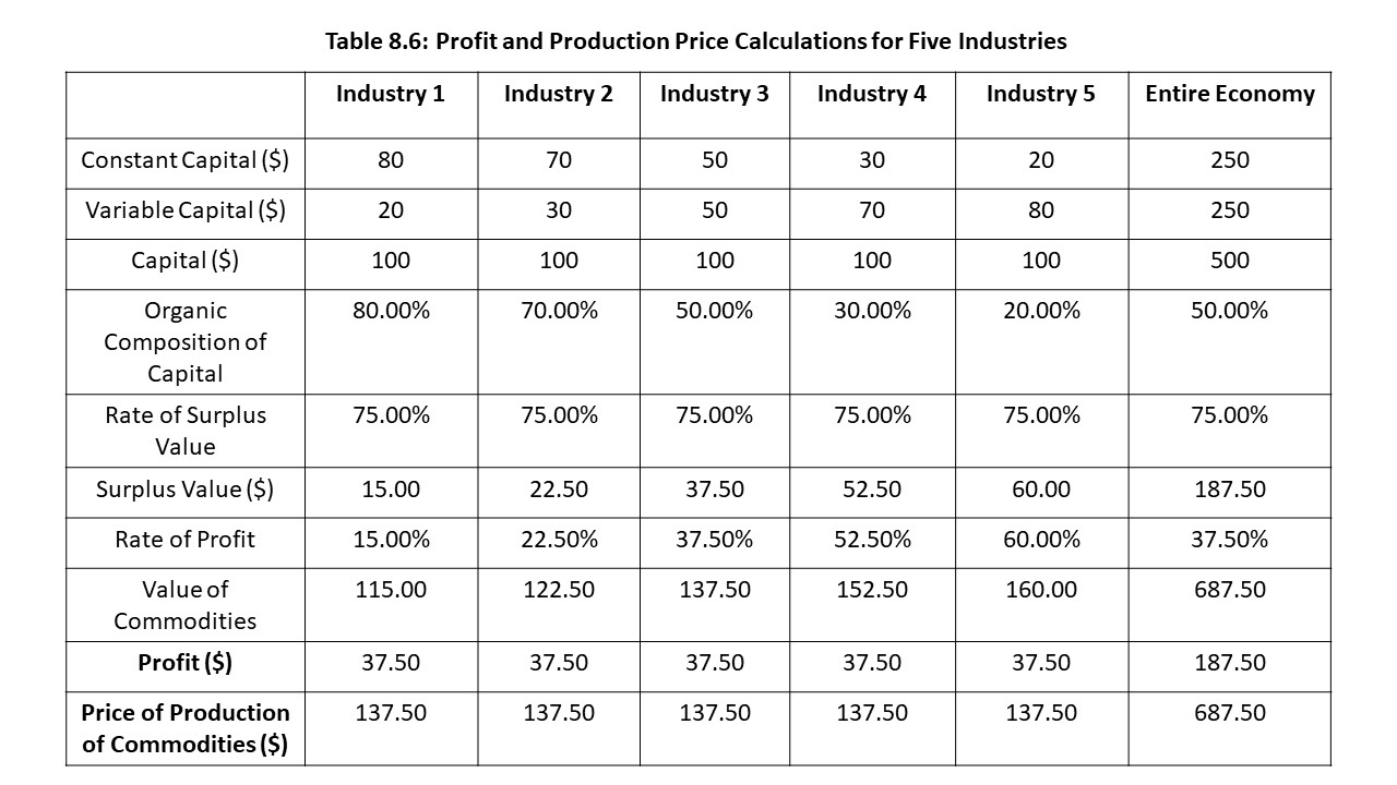
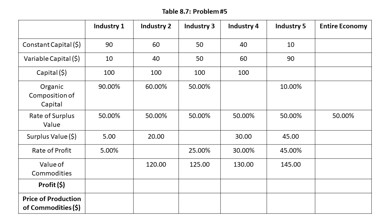
Because all capital should earn the same rate of profit in a competitive capitalist economy, we can multiply the amount of capital invested in each industry by r to obtain the averageprofit that will be appropriated in each industry. Because the capital invested in each industry is the same ($100) and the general rate of profit is the same (r), the profit appropriated in each industry is the same in this example. Table 8.6 adds two additional rows of information to the information from Table 8.5 that applies specifically to this question of profit rate equalization.
Table 8.6 shows that the profit in each industry is $37.50. The reader should notice that the concept of profit is one that we have not yet discussed in the Marxian framework. It is not the same as surplus value. In fact, the equalization of the profit rate has created a situation in which the profits received and the surplus values produced are different in most of the industries in the table. In addition, the selling prices of the commodities will now be different from the values of the commodities. That is, the prices of production in each industry are equal to the total capital advanced in that industry plus the profits received in that industry.
From a dynamic perspective, we can say that capital flows out of low profit industries and into high profit industries. As capital moves, production in high profit industries increases. The increased production causes the market price of the commodities produced in those industries to fall below the market value of those commodities.[4] As a result, the profit rates fall in high profit industries. Similarly, production in low profit industries contracts as capital flows out of them. The decrease in production causes the market price of the commodities in those industries to rise above the market value of those commodities. As a result, the profit rates increase in low profit industries. Capital movements will continue to occur until the profit rates have equalized across all industries. In addition, we can see from Table 8.6 that prices of production rise above their values in low profit industries and fall below their values in high profit industries. Only Industry 3, which possesses the same OCC as the entire economy, earns a profit equal to the surplus value it produces and charges a price of production equal to the value of its commodities.
It is important not to become lost in the details and miss the fact that this analysis of competitive capitalism assigns a central role to class exploitation. It is the working class that produces the surplus value. Even though each industry ends up earning an amount of profit that is different from the surplus value it produces (except for Industry 3), the aggregate surplus value for the entire economy ($187.50) is equal to the aggregate profit. In other words, the capitalist class shares equally in the mass of surplus value produced by the working class according to each capitalist’s share of the total capital. In addition, the aggregate value of the commodities produced depends upon the SNALT required for their production within the Marxian framework. As Table 8.6 shows, the aggregate value of $687.50 is the same as the aggregate production price of the commodities produced for the entire economy. Marx identified these two key aggregate equalities in volume III of Capital which we can summarize as follows:
The major objection to this Marxian analysis has been dubbed the Transformation Problem. The problem is easy enough to grasp but has proven incredibly difficult to solve to the satisfaction of all those interested in this question. The problem is that the elements of constant and variable capital also have values that must be transformed into production prices. In our example, these values have been left in their original form, giving rise to the objection that the transformation of values into production prices is not complete. For example, in Industry 1 constant capital might be advanced for the purchase of iron ore to be used in production. It will be purchased at its value, but once the profit rate has equalized, it should be purchased at its production price rather than its value. Many proposed solutions to this problem have been put forward since the late nineteenth century. The problem is that no one has yet discovered a way to transform the input values into production prices while at the same time maintaining both of Marx’s aggregate equalities. This problem continues to be one of the most challenging problems in the history of economic thought. Despite this problem, Marxian analysis provides a powerful explanation for the equalization of profit rates in capitalist economies within the context of a framework that grants a central place to the class struggle between workers and capitalists.
For many sellers, a fall in the price of their product can create extreme economic hardship. For example, Kevin Sieff explains that the steep drop in the price of coffee in the past few years has placed coffee growers in Guatemala under great economic pressure. Consequently, Sieff reports that many farmers have decided to migrate to the United States, as they have been operating at a loss due to an approximately 60% drop in the price of coffee. The decision to operate at a loss suggests that the price is below average total cost but at least as high as average variable cost. In other words, coffee growers are earning enough revenue to cover their total variable cost of production and probably part, but not all, of their fixed cost of production. In other cases, coffee growers shut down entirely because prices are below their average variable cost of production. As Sieff explains, “[a]bandoned coffee farms lie fallow along the dirt roads that wind through the region.” Part of the problem facing Guatemalan coffee growers is a rise in production costs. Sieff explains that smaller coffee farmers have been required to purchase chemicals to address the problem of “coffee rust,” which is a fungus. The rise in costs pushes up average variable cost. At the same time, Sieff explains that coffee prices are falling due to increased production in Brazil, Vietnam, Honduras, and Colombia. The combination of rising average variable cost and falling product prices is responsible for many coffee growers operating at a loss or shutting down altogether. Because different coffee growers have different average variable costs, some can avoid shutting down, but others are not so lucky. Sieff reports that Guatemalan farmers have recently been paid a price of $1.20 per pound while their average total cost is estimated to be $1.93 per pound. Sieff explains that this situation represents a sharp break from 2012 when coffee prices were $2 per pound, and production was profitable. In that case, we can conclude that price had exceeded average total cost, but that lucrative scenario is now firmly in the past.
Summary of Key Points
Economic profit is typically smaller than accounting profit because economic profit subtracts both explicit costs and implicit costs from total revenue.
A firm earns a normal profit when its economic profit is zero.
Neoclassical economists regard perfectly competitive markets as the normative ideal among market structures.
Firms in a perfectly competitive market structure are price-takers, and so average revenue and marginal revenue are equal to price.
To maximize economic profit in the short run, a perfectly competitive firm must produce such that price equals marginal cost and should only produce a positive output level when price is greater than or equal to average variable cost.
The short run supply curve of a perfectly competitive firm is the marginal cost curve above the minimum average variable cost of production.
In the long run, economic profits will be driven to zero as firms enter due to positive short run economic profits and as they exit due to negative short run economic profits.
The long run industry supply curve may be positively sloped, negatively sloped, or horizontal depending on the way in which input prices react as new firms enter an industry.
Neoclassical economists conclude that perfect competition leads to economic efficiency, but they do not emphasize the distinction between market demand and needs, the power struggle between social classes, and the fact that people’s happiness might depend as much on the work that they do as on the material consumption they enjoy.
In Marxian analysis, rates of profit differ across industries due to differing organic compositions of capital.
Capital moves between industries in search of the highest profit rate until production prices are formed, and the general rate of profit is established across all sectors.
The Transformation Problem exists because many believe that the values of inputs must be transformed into production prices in the same way that the values of final commodities are transformed into production prices.
List of Key Terms
Average revenue (AR)
Marginal revenue (MR)
Accounting profit
Explicit costs
Implicit costs
Economic profit
Normal profit
Market structure
Market power
Market power spectrum
Perfect competition
Price-taker
Long run marginal cost (LRMC)
Optimal plant size
Long run industry supply (LRIS)
Constant-cost industry
Increasing-cost industry
Decreasing-cost industry
Organic composition of capital (OCC)
General rate of profit (r)
Average profit
Prices of production
Transformation problem
Problems for Review
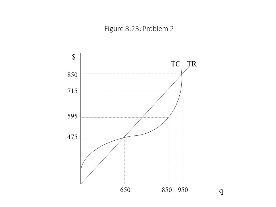
1.Suppose the market for frozen pizza is perfectly competitive and the current market price of a frozen pizza is $5.75. On a graph, draw the total revenue curve facing one firm in the market as well as the new total revenue curve when the market price rises to $6.25 per frozen pizza. Place dollars ($) on the vertical axis and quantity (q) on the horizontal axis.
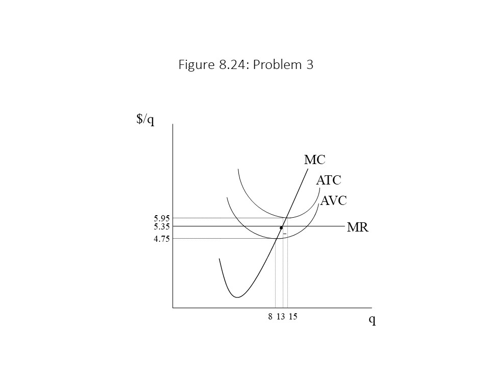
Figure 8.24 maximizes its economic profit.
What is the profit-maximizing output level and price?
What is total revenue?
What is total economic cost?
What is total economic profit?
What is the total fixed cost?
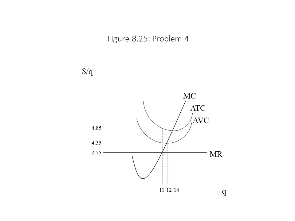
4. Answer the following questions when the firm represented in Figure 8.25 maximizes its economic profit.
What is the profit-maximizing output level and price?
What is total revenue?
What is total economic cost?
What is total economic profit?
What is the total fixed cost?
5. Complete the remainder of Table 8.7 using the given information. What is the general rate of profit? Do Marx’s two aggregate equalities hold?
It was my experience as a teaching assistant for Prof. Thomas R. Swartz at the University of Notre Dame in the early 2000s that inspired my approach to the derivation of LRIS curves in this section. ↵
In Table 8.5, the total surplus value may be calculated as the product of the rate of surplus value (s/v) and the variable capital (v). The rate of profit is calculated as s/(c+v) as in Chapter 4. Finally, the total value of the commodities produced in each industry is calculated as the sum of c, v, and s, which is also how the total value was calculated in Chapter 4. ↵
Recall from Chapter 4 that fluctuations in supply and demand can cause the value of a commodity and its price to diverge. ↵
Sieff, Kevin. “Falling Coffee Prices Drive Guatemalan migration to the United States.” The Washington Post. 11 June 2019. ↵


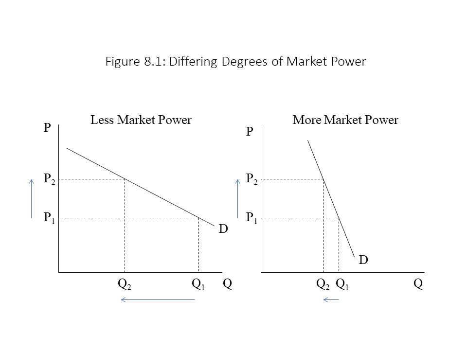 The firm facing a flatter demand curve possesses less market power because the rise in price from P1 to P2 leads to a much sharper reduction in quantity demanded. The firm facing a steeper demand curve possesses considerable market power.
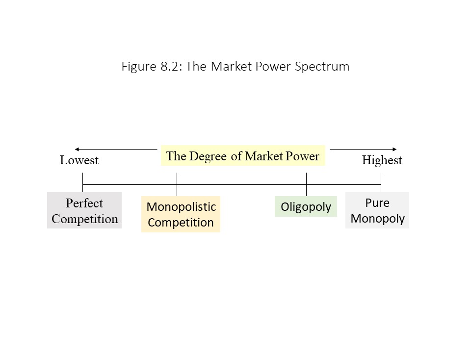 Each of these market structures is distinguished along the lines of the three dimensions mentioned previously. The only market structure that we will examine in this chapter is perfect competition. According to neoclassical economists, a perfectly competitive market structure has the following three characteristics:
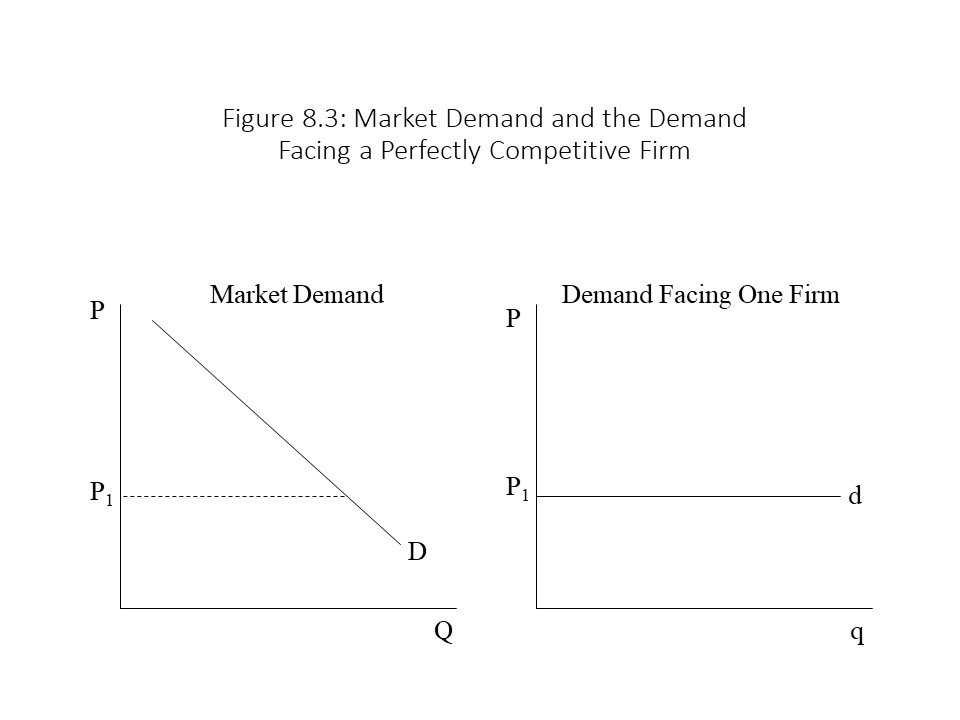 The reason for the difference is that the individual perfectly competitive firm is a price-taker and only faces a tiny segment (d) of the entire market demand (D). If the perfectly competitive firm attempts to raise the price above P1, then the quantity demanded (q) will fall to 0 units because every buyer can obtain a perfect substitute from a competitor at a price of P1. Additionally, it makes no sense for the firm to reduce the price below P1 because the firm can sell as much as it wants at the market price. It will sacrifice revenue needlessly if it cuts price because a price cut is not necessary to sell additional units. The firm is so small relative to the entire market that plenty of customers exist at the market price. We can also state that demand is infinitely elastic in the case of the demand curve facing the perfectly competitive firm. The smallest price increase will cause quantity demanded to fall to zero, and the smallest price cut will cause quantity demanded to soar.
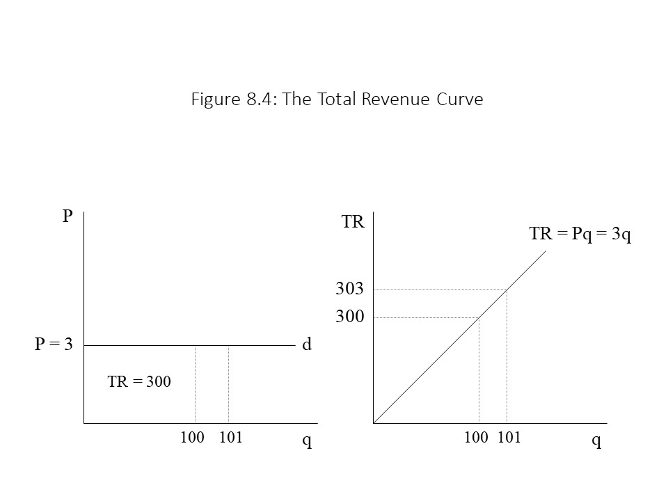 The graph on the left in Figure 8.4 shows that the area of the box under the demand curve is equal to total revenue since it is calculated as the product of price and quantity demanded. Furthermore, an additional unit can be sold at a price of $3 because the firm is a price-taker. The graph on the right shows what happens to total revenue as the quantity sold rises. It increases in a linear fashion because with each additional unit sold, the TR rises by the amount of the price of that unit, which is constant since the firm is a price-taker. Hence, the 101st unit raises TR from $300 to $303.
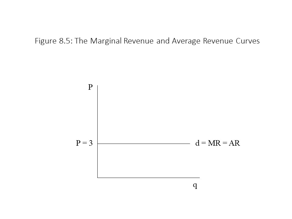 All the revenue measures can also be expressed in tabular form as shown in Table 8.2.
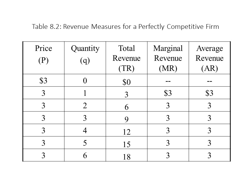
 According to Table 8.3, the firm will maximize its economic profit by producing 600 units of output. At that output level, its economic profit will be $970. One can also see that if the firm produces too little or too much, then it will experience economic losses. Producing too little means that the firm fails to take sufficient advantage of labor specialization and the division of labor. Producing too much means that the firm fails to recognize the negative impact that diminishing returns to labor carries for profitability.
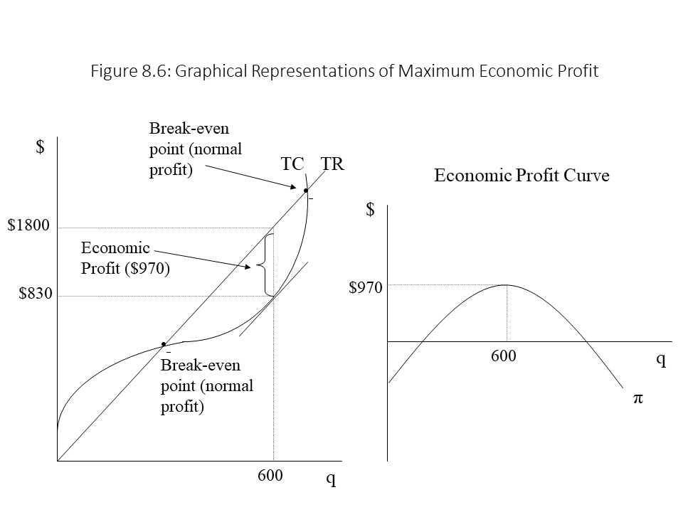 Figure 8.6 shows that economic losses exist to the left of the first break-even point because TC exceeds TR. At the break-even point, TC = TR and so economic profit is $0. Earlier in the chapter, it was argued that an economic profit of zero is still acceptable to the firm because all costs are covered. Because the opportunity costs are covered as well, the firm earns a normal profit. In between the two break-even points, the firm’s revenues exceed its costs. Therefore, positive economic profits are earned over that range of output. At a single output level, however, the gap between the TR and the TC is maximized. At that point where Q = 600 units, the economic profit is at a maximum.
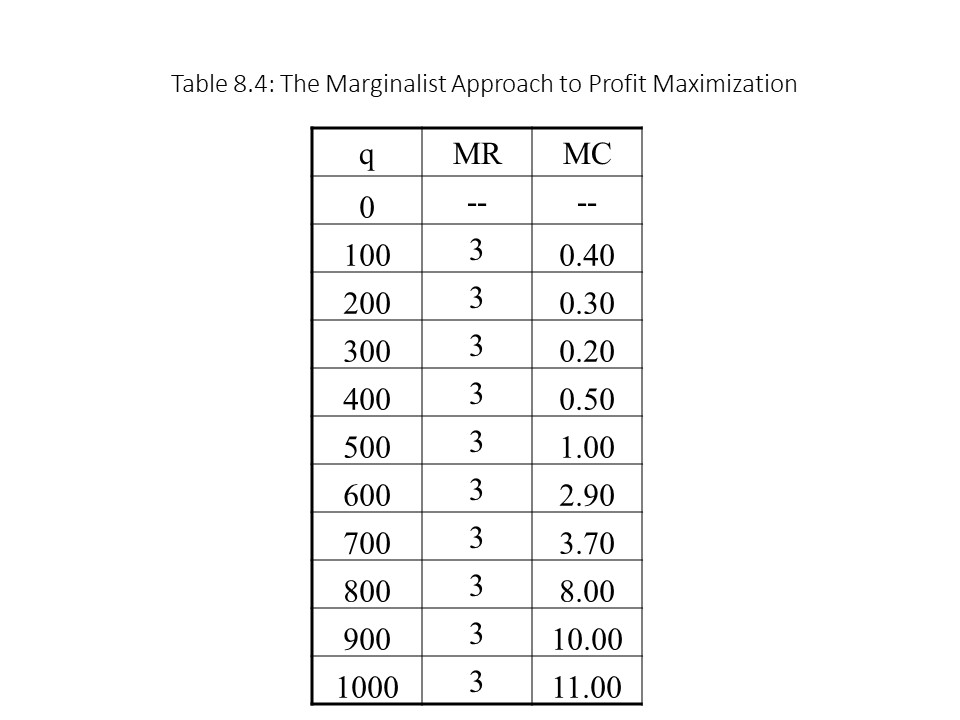
 We can summarize how these marginal adjustments lead to the profit-maximizing choice of output:
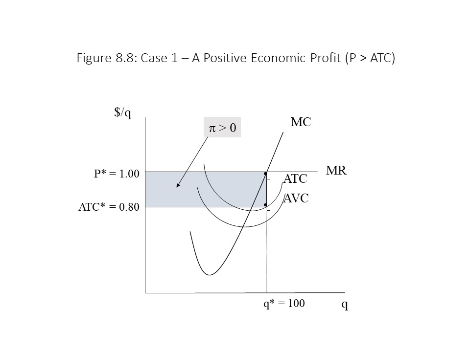 We begin our analysis of this case by finding the point at which MR = MC. Moving straight down from the intersection of these two curves to the horizontal axis gives us an output level of 100 units. Before we declare this output level to be the profit-maximizing choice, we need to check whether P ≥ AVC. In this case, it is greater. Even though the specific AVC has not been identified in the graph, we know that P exceeds AVC because at q* the MR curve is higher than the AVC curve. Therefore, the profit-maximizing output level is 100 units.
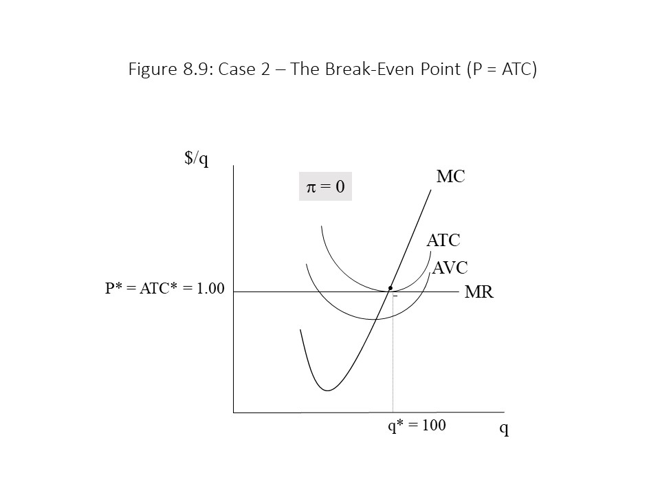 Again, we find the intersection of MR and MC to occur at 100 units of output. In addition, at that output level, the MR curve lies above the AVC curve and so the firm will operate. The profit-maximizing output level is 100 units as before. The TR in this case is $100 (= $1.00 per unit times 100 units). Because the ATC is also $1.00 per unit, the TC in this case is $100 as well. As a result, the economic profit is zero. Another way to see why economic profit is equal to zero is to notice that the box representing TR in the graph also represents TC. The reader should recall that the firm earns a normal profit in this case, and so this situation is not unacceptable to the firm. That is, the firm could not earn a greater profit in any other industry.
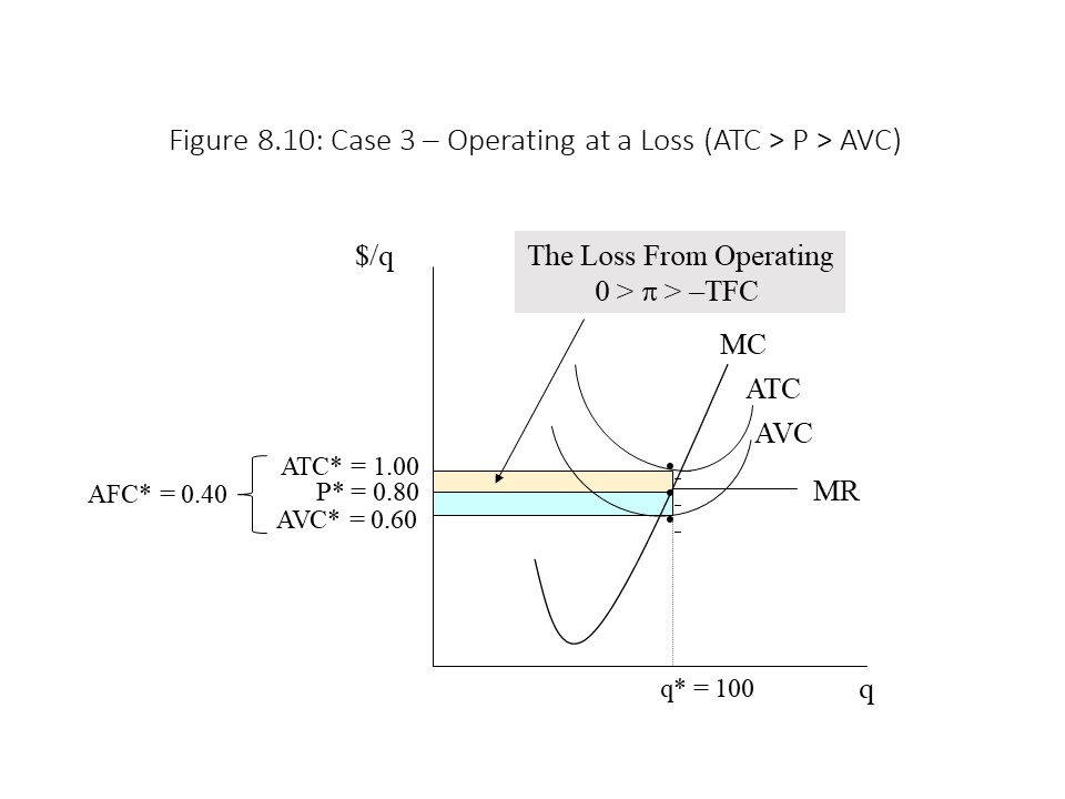 That is, shutting down is an even worse option. Let’s see why. The intersection of MR and MC occurs at 100 units of output as before and P = $0.80 is clearly above AVC = $0.60 at that output level. Hence, the firm will operate. The firm’s TR is equal to $80 (= $0.80 per unit times 100 units) and the firm’s TC is equal to $100 (= $1.00 per unit times 100 units). The firm’s economic profit is, therefore, equal to -$20 (= $80 minus $100). This loss is represented in Figure 8.10 as the top shaded box.
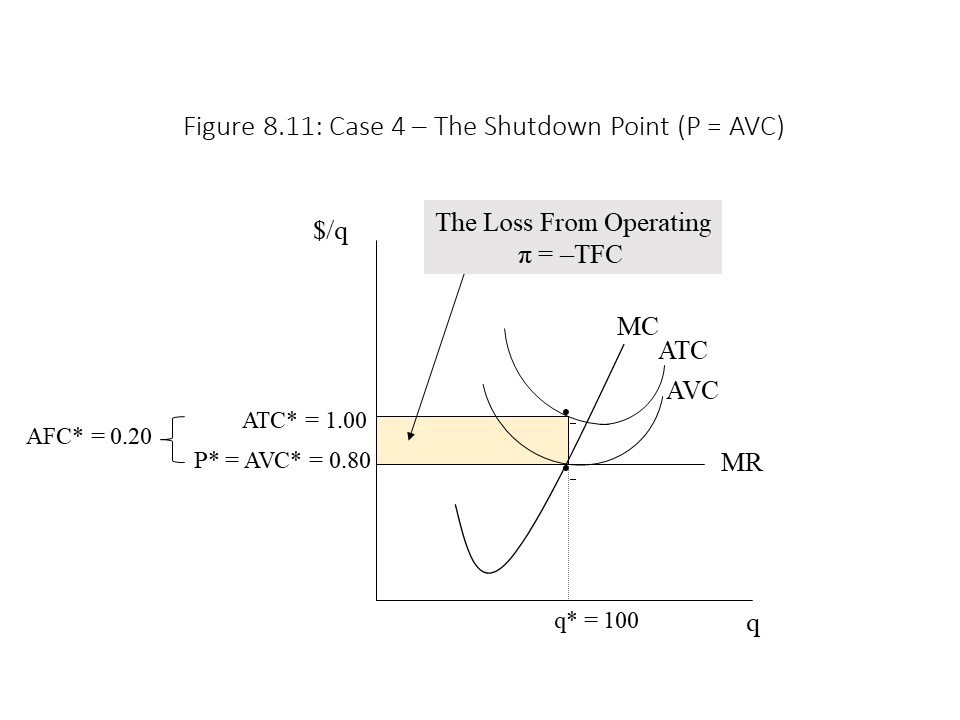 In this case, the intersection between MR and MC occurs at 100 units of output as before. The price, however, is exactly equal to AVC at this output level. The second rule of profit maximization requires that price be greater than or equal to AVC for the firm to operate. This condition is fulfilled and so the firm will operate. We can also see that TR is equal to $80 (= $0.80 per unit times 100 units) and TC is equal to $100 (= $1.00 per unit times 100 units). The firm’s economic profit is, therefore, equal to -$20 (= $80 – $100). In addition, because the AFC = $0.20 per unit, the TFC = $20 (= $0.20 per unit times 100 units). If the firm shuts down then, its economic profit will be equal to -$20 (= –TFC). Clearly, the profit from operating is the same as the profit from shutting down. Because the firm is indifferent between operating and shutting down, by convention, we conclude that the firm will operate.
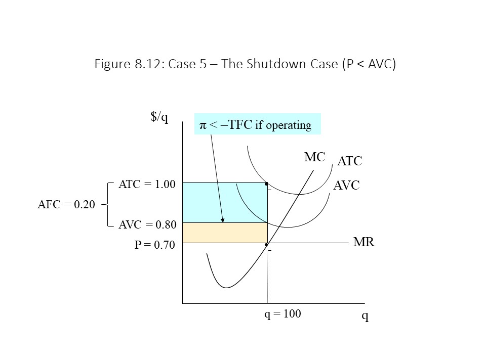 Again, the MR = MC intersection occurs at 100 units of output, but this time, the price of $0.70 per unit is below the AVC of $0.80 per unit. The second rule of profit maximization indicates that the firm should shut down in this case. The economic profit in this case is equal to –TFC. Because the AFC is $0.20 per unit, the TFC equals $20 (= $0.20 per unit times 100 units). The economic profit is, therefore, -$20. The careful reader might wonder how we can calculate TFC at an output level of 100 units when the firm has opted to produce zero units. The reason is that TFC is the same at all output levels so if we determine the TFC at 100 units of output, we also know the TFC at zero units of output.
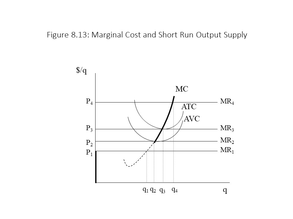 As the market price falls, the MR curve shifts downward. At the highest price of P4, the two rules of profit maximization indicate that q4 should be produced. At that output level, MR = MC and P > AVC. When the price declines to P3, the firm will produce q3, and the break-even point will be reached since P = ATC. When the price declines further to P2, q2 is produced and the shutdown point is reached since P = AVC. Finally, when the price falls to P1, the firm maximizes its economic profit by shutting down and producing zero units of output because P < AVC. This analysis has allowed us to observe the different quantities of output supplied at different market prices, other factors held constant. In other words, the short run analysis of profit maximization has made possible the derivation of the firm’s output supply curve. Because the intersections of MR with MC determine the profit-maximizing output levels, we can conclude that the supply curve is the MC curve above the minimum AVC. In Figure 8.13, the supply curve is the darkened portion of the MC curve plus the vertical axis below the minimum AVC because the firm produces zero units of output when the market price falls below that level.
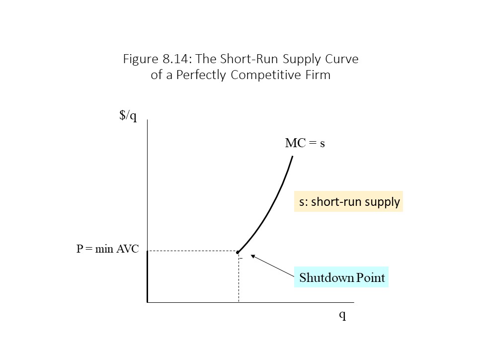 This analysis reveals the reason why we drew the supply curves in chapter 3 as suspended without a vertical intercept. We can also reinterpret the market supply curve. In chapter 3, it was explained that the market supply curve is the aggregation of many individual sellers’ supply curves, which we can obtain through horizontal summation. We now see that the market supply curve is also the horizontal summation of the individual firms’ MC curves.
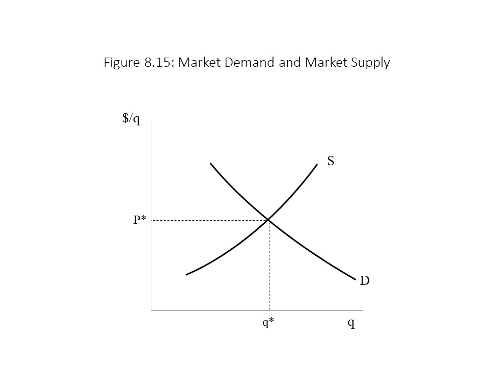
 Why does this case represent the long run equilibrium outcome? The reason is that short run deviations from this situation produce an inherent long run tendency to change in the direction of this outcome. For example, in Figure 8.17, the market price and quantity exchanged begin at P1 and Q1, and the firm produces q1 units of output.
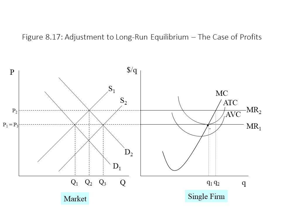 Now assume that a short run increase in demand causes the demand curve to shift to D2. The increase in the market price to P2 causes the firm’s MR curve to shift upwards from MR1 to MR2. The firm’s profit-maximizing choice of output, therefore, rises from q1 to q2. The price charged now exceeds ATC resulting in positive economic profits. In the long run, firms outside the industry respond to the resulting economic profits, which function as a signal that they should enter this industry. As the number of sellers in the industry increases, the market supply curve shifts rightward from S1 to S2. The market price falls to P3, and the economic profits return to zero as the firm reduces output to the original level of q1. It should be noted that the market price returns to its original level, but the market quantity exchanged has increased from Q1 to Q3. This result is argued to be consistent with Adam Smith’s Invisible Hand in that the free market has reallocated a part of society’s resources toward the production of this product for which consumer demand has grown.
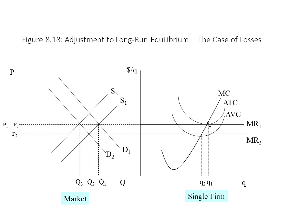 The decrease in the market price to P2 causes the firm’s MR curve to shift downwards from MR1 to MR2. The firm’s profit-maximizing choice of output, therefore, falls from q1 to q2. The price charged is now below ATC resulting in economic losses. In the long run, firms inside the industry respond to the economic losses, which function as a signal that they should exit this industry. As the number of sellers in the industry decreases, the market supply curve shifts leftward from S1 to S2. The market price rises to P3, and the economic profits return to zero as the firm increases output to the original level of q1. It should be noted that the market price returns to its original level, but the market quantity exchanged has decreased from Q1 to Q3. This result is also argued to be consistent with Adam Smith’s Invisible Hand in that the free market has reallocated a part of society’s resources away from the production of this product for which consumer demand has fallen.