5.2: Descriptive statistics for nominal data

Most examples we have looked at so far in this book involved two nominal variables: the independent variable VARIETY (with the values BRITISH ENGLISH vs. AMERICAN ENGLISH) and a dependent variable consisting of some linguistic alternation (mostly regional synonyms of some lexicalized concept). Thus, this kind of research design should already be somewhat familiar.

For a closer look, we will apply it to the first of the three hypotheses introduced in the preceding section, which is restated here with the background assumption from which it is derived:

(9) Assumption: Discourse-old items occur before discourse-new items.

Hypothesis: The S-POSSESSIVE will be used when the modifier is DISCOURSE-OLD, the OF-POSSESSIVE will be used when the modifier is DISCOURSE-NEW.

Note that the terms S-POSSESSIVE and OF-POSSESSIVE are typeset in small caps in these hypotheses. This is done in order to show that they are values of a variable in a particular research design, based on a particular theoretical construct. As such, these values must, of course, be given operational definitions (also, the construct upon which the variable is based should be explicated with reference to a particular model of language, but this would lead us too far from the purpose of this chapter and so I will assume that the phenomenon “English nominal possession” is self-explanatory).

The definitions I used were the following:

(10) a. S-POSSESSIVE: A construction consisting of a possessive pronoun or a noun phrase marked by the clitic ’s modifying a noun following it, where the construction as a whole is not a proper name.

b. OF-POSSESSIVE: A construction consisting of a noun modified by a prepositional phrase with of, where the construction as a whole encodes a relation that could theoretically also be encoded by the s-possessive and is not a proper name

Proper names (such as Scotty’s Bar or District of Columbia) are excluded in both cases because they are fixed and could not vary. Therefore, they will not be subject to any restrictions concerning givenness, animacy or length.

To turn these definitions into operational definitions, we need to provide the specific queries used to extract the data, including a description of those aspects of corpus annotation used in formulating these queries. We also need annotation schemes detailing how to distinguish proper names from other uses and how to identify of -constructions that encode relations that could also be encoded by the s -possessive.

The s -possessive is easy to extract if we use the tagging present in the BROWN corpus: words with the possessive clitic (i.e. ’s, or just ’ for words whose stem ends in s) as well as possessive pronouns are annotated with tags ending in the dollar sign $, so a query for words tagged in this way will retrieve all cases with high precision and recall. For the of -possessive, extraction is more difficult – the safest way seems to be to search for words tagged as nouns followed by the preposition of, which already excludes uses like [most of NP] (where the quantifying expression is tagged as a post-determiner) [because of NP], [afraid of NP], etc.

The annotation of the results for proper name or common noun status can be done in various ways – in some corpora (but not in the BROWN corpus), the POS tags may help, in others, we might use capitalization as a hint, etc. The annotation for whether or not an of -construction encodes a relation that could also be encoded by an s -possessive can be done as discussed in Section 4.2.3 of Chapter 4.

Using these operationalizations for the purposes of the case studies in this chapter, I retrieved and annotated a one-percent sample of each construction (the constructions are so frequent that even one percent leaves us with 222 s -and 178 of -possessives (the full data set for the studies presented in this and the following two subsections can be found in the Supplementary Online Material, file HKD3).

Next, the values DISCOURSE-OLD and DISCOURSE-NEW have to be operationalized. This could be done using the measure of referential distance discussed in Section 3.2 of Chapter 3, which (in slightly different versions) is the most frequently used operationalization in corpus linguistics. Since we want to demonstrate a design with two nominal variables, however, and in order to illustrate that constructs can be operationalized in different ways, I will use a different, somewhat indirect operationalization. It is well established that pronouns tend to refer to old information, whereas new information must be introduced using common nouns in full lexical NPs. Thus, we can assume a correlation between the construct discourse-old and the construct pronoun on the one hand, and the construct discourse-new and the construct common noun on the other.

This correlation is not perfect, as common nouns can also encode old information, so using PART OF SPEECH OF NOMINAL EXPRESSION as an operational definition for Givenness is somewhat crude in terms of validity, but the advantage is that it yields a highly reliable, easy-to-annotate definition: we can use the part-of-speech tagging to annotate our sample automatically.

We can now state the following quantitative prediction based on our hypothesis:

(11) Prediction: There will be more cases of the S-POESSESSIVE with DISCOURSE-OLD modifiers than with DISCOURSE-NEW modifiers, and more cases of the OF-POSSESSIVE with discourse-new modifiers than with DISCOURSE-OLD modifiers.

Table 5.1 shows the absolute frequencies of the parts of speech of the modifier in both constructions (examples with proper names were discarded, as the givenness of proper names in discourse is less predictable than that of pronouns and common nouns).

Such a table, examples of which we have already seen in previous chapters, is referred to as a contingency table. In this case, the contingency table consists of four cells showing the frequencies of the four intersections of the variables GIVENESS, (with the values NEW, i.e. “pronoun”, and OLD, i.e. “common noun” and POSSESSIVE (with the values S and OF); in other words, it is a two-by-two table. Possessive is presented as the dependent variable here, since logically the hypothesis is that the information status of the modifier influences the choice of construction, but mathematically it does not matter in contingency tables what we treat as the dependent or independent variable.

Table 5.1: Part of speech of the modifier in the s -possessive and the of -possessive

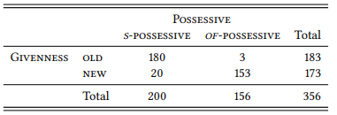
In addition, there are two cells showing the row totals (the sum of all cells in a given row) and the column totals (the sum of all cells in a given column), and one cell showing the table total (the sum of all four intersections). The row and column totals for a given cell are referred to as the marginal frequencies for that cell.

5.2.1 Percentages

The frequencies in Table 5.1 are fairly easy to interpret in this case, because the differences in frequency are very clear. However, we should be wary of basing our assesment of corpus data directly on raw frequencies in a contingency table. These can be very misleading, especially if the marginal frequencies of the variables differ substantially, which in this case, they do: the s -possessive is more frequent overall than the of -possessive and discourse-old modifiers (i.e., pronouns) are slightly more frequent overall than discourse-new ones (i.e., common nouns).

Thus, it is generally useful to convert the absolute frequencies to relative frequencies, abstracting away from the differences in marginal frequencies. In order to convert an absolute frequency n into a relative one, we simply divide it by the total number of cases N of which it is a part. This gives us a decimal fraction expressing the frequency as a proportion of 1. If we want a percentage instead, we multiply this decimal fraction by 100, thus expressing our frequency as a proportion of 100.

For example, if we have a group of 31 students studying some foreign language and six of them study German, the percentage of students studying German is

Multiplying this by 100, we get

In other words, a percentage is just another way of expressing a decimal fraction, which is just another way of expressing a fraction, all of which are (among other things) ways of expressing relative frequencies (i.e., proportions). In academic papers, it is common to report relative frequencies as decimal fractions rather than as percentages, so we will follow this practice here.

If we want to convert the absolute frequencies in Table 5.1 into relative frequencies, we first have to decide what the relevant total N is. There are three possibilities, all of which are useful in some way: we can divide each cell by its column total, by its row total or by the table total. Table 5.2 shows the results for all three possibilities.

The column proportions can be related to our prediction most straightforwardly: based on our hypothesis, we predicted that in our sample a majority of s -possessives should have modifiers that refer to discourse-old information and, conversely a majority of of -possessives should have modifiers that refer to discourse-new information.

The relevance of the row proportions is less clear in this case. We might predict, based on our hypothesis, that the majority of modifiers referring to old information should occur in s -possessives and the majority of modifiers referring to new information should occur in of -possessives.

This is the case in Table 5.2, and this is certainly compatible with our hypothesis. However, if it were not the case, this could also be compatible with our hypothesis. Note that the constructions differ in frequency, with the of -possessive being only three-quarters as frequent as the s -possessive. Now imagine the difference was ten to one instead of four to three. In this case, we might well find that the majority of both old and new modifiers occurs in the s -possessives, simply because there are so many more s-possessives than of -possessives. We would, however, expect the majority to be larger in the case of old modifiers than in the case of new modifiers. In other words, even if we are looking at row percentages, the relevant comparisons are across rows, not within rows.

Table 5.2: Absolute and relative frequencies of the modifier’s givenness (as reflected in its part of speech) in the English possessive constructions

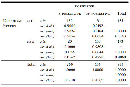
Whether column or row proportions are more relevant to a hypothesis depends, of course, on the way variables are arranged in the table: if we rotate the table such that the variable POSESSIVE ends up in the rows, then the row proportions would be more relevant. When interpreting proportions in a contingency table, we have to find those that actually relate to our hypothesis. In any case, the interpretation of both row and column proportions requires us to choose one value of one of our variables and compare it across the two values of the other variable, and then compare this comparison to a comparison of the other value of that variable. If that sounds complicated, this is because it is complicated.

It would be less confusing if we had a way of taking into account both values of both variables at the same time. The table proportions allow this to some extent. The way our hypothesis is phrased, we would expect a majority of cases to instantiate the intersections S -POSSESSIVE ∩ DISCOURSE-OLD and OF -POSSESSIVE ∩ DISCOURSE-NEW, with a minority of cases instantiating the other two intersections. In Table 5.2, this is clearly the case: the intersection S -POSSESSIVE ∩ DISCOURSE-OLD contains more than fifty percent of all cases, the intersection OF -POSSESSIVE ∩ DISCOURSE-NEW well over 40 percent. Again, if the marginal frequencies differ more extremely, so may the table percentages in the relevant intersections. We could imagine a situation, for example, where 90 percent of the cases fell into the intersection S -POSSESSIVE ∩ DISCOURSE-OLD and 10 percent in the intersection OF -POSSESSIVE ∩ DISCOURSE-NEW – this would still be a corroboratation of our hypothesis.

While relative frequencies (whether expressed as decimal fractions or as percentages) are, with due care, more easily interpretable than absolute frequencies, they have two disadvantages. First, by abstracting away from the absolute frequencies, we lose valuable information: we would interpret a distribution such as that in Table 5.3 differently, if we knew that it was based on a sample on just 35 instead of 356 corpus hits. Second, it provides no sense of how different our observed distribution is from the distribution that we would expect if there was no relation between our two variables, i.e., if the values were distributed randomly. Thus, instead of (or in addition to) using relative frequencies, we should compare the observed absolute frequencies of the intersections of our variables with the expected absolute frequencies, i.e., the absolute frequencies we would expect if there was a random relationship between the variables. This comparison between observed and expected frequencies also provides a foundation for inferential statistics, discussed in Chapter 6.

5.2.2 Observed and expected frequencies

So how do we determine the expected frequencies of the intersections of our variables? Consider the textbook example of a random process: flipping a coin onto a hard surface. Ignoring the theoretical and extremely remote possibility that the coin will land, and remain standing, on its edge, there are two possible outcomes, heads and tails. If the coin has not been manipulated in some clever way, for example, by making one side heavier than the other, the probability for heads and tails is 0.5 (or fifty percent) each (such a coin is called a fair coin in statistics).

From these probabilities, we can calculate the expected frequency of heads and tails in a series of coin flips. If we flip the coin ten times, we expect five heads and five tails, because 0.5×10 = 5. If we flip the coin 42 times, the expected frequency is 21 for heads and 21 for tails (0.5 × 42), and so on. In the real world, we would of course expect some variation (more on this in Chapter 6), so expected frequency refers to a theoretical expectation derived by multiplying the probability of an event by the total number of observations.

So how do we transfer this logic to a contingency table like Table 5.1? Naively, we might assume that the expected frequencies for each cell can be determined by taking the total number of observations and dividing it by four: if the data were distributed randomly, each intersection of values should have about the same frequency (just like, when tossing a coin, each side should come up roughly the same number of times). However, this would only be the case if all marginal frequencies were the same, for example, if our sample contained fifty S -POSSESSIVES and fifty OF -POSSESSIVES and fifty of the modifiers were discourse old (i.e. pronouns) and fifty of them were discourse-new (i.e. common nouns). But this is not the case: there are more discourse-old modifiers than discourse-new ones (183 vs. 173) and there are more s -possessives than of -possessives (200 vs. 156).

These marginal frequencies of our variables and their values are a fact about our data that must be taken as a given when calculating the expected frequencies: our hypothesis says nothing about the overall frequency of the two constructions or the overall frequency of discourse-old and discourse-new modifiers, but only about the frequencies with which these values should co-occur. In other words, the question we must answer is the following: Given that the s - and the of -possessive occur 200 and 156 times respectively and given that there are 183 discourse-old modifiers and 173 discourse-new modifiers, how frequently would each combination these values occur by chance?

Put like this, the answer is conceptually quite simple: the marginal frequencies should be distributed across the intersections of our variables such that the relative frequencies in each row should be the same as those of the row total and the relative frequencies in each column should be the same as those of the column total.

For example, 56.18 percent of all possessive constructions in our sample are s -possessives and 43.82 percent are of -possessives; if there were a random relationship between type of construction and givenness of the modifier, we should find the same proportions for the 183 constructions with old modifiers, i.e. 183 × 0.5618 = 102.81 s -possessives and 183 × 0.4382 = 80.19 of -possessives. Likewise, there are 173 constructions with new modifiers, so 173 × 0.5618 = 97.19 of them should be s -possessives and 173 × 0.4382 = 75.81 of them should be of -possessives. The same goes for the columns: 51.4 percent of all constructions have old modifiers and 41.6 percent have new modifiers. If there were a random relationship between type of construction and givenness of the modifier, we should find the same proportions for both types of possessive construction: there should be 200 × 0.514 = 102.8 s -possessives with old modifiers and 97.2 with new modifiers, as well as 156 × 0.514 = 80.18 of -possessives with old modifiers and 156 × 0.486 = 75.82 of -possessives with new modifiers. Note that the expected frequencies for each intersection are the same whether we use the total row percentages or the total column percentages: the small differences are due to rounding errors.

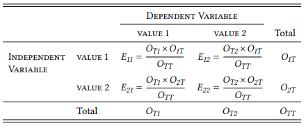
To avoid rounding errors, we should not actually convert the row and column totals to percentages at all, but use the following much simpler way of calculating the expected frequencies: for each cell, we simply multiply its marginal frequencies and divide the result by the table total as shown in Table 5.3; note that we are using the standard convention of using O to refer to observed frequencies, E to refer to expected frequencies, and subscripts to refer to rows and columns. The convention for these subscripts is as follows: use 1 for the first row or column, 2 for the second row or column, and T for the row or column total, and give the index for the row before that of the column. For example, E₂₁ refers to the expected frequency of the cell in the second row and the first column, O_1T refers to the total of the first row, and so on.

Table 5.3: Calculating expected frequencies from observed frequencies

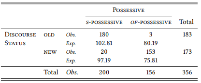
Applying this procedure to our observed frequencies yields the results shown in Table 5.4. One should always report nominal data in this way, i.e., giving both the observed and the expected frequencies in the form of a contingency table.

We can now compare the observed and expected frequencies of each intersection to see whether the difference conforms to our quantitative prediction. This is clearly the case: for the intersections OF -POSSESSIVE ∩ DISCOURSE-NEW and OF -POSSESSIVE ∩ DISCOURSE-NEW, the observed frequencies are higher than the expected ones, for the intersections OF -POSSESSIVE ∩ DISCOURSE-NEW and OF -POSSESSIVE ∩ DISCOURSE-NEW, the observed frequencies are lower than the expected ones.

This conditional distribution seems to corroborate our hypothesis. However, note that it does not yet prove or disprove anything, since, as mentioned above, we would never expect a real-world distribution of events to match the expected distribution perfectly. We will return to this issue in Chapter 6.

Table 5.4: Observed and expected frequencies of old and new modifiers in the s - and the of -possessive