6.2: Probabilities and significance testing

Recall the example of a coin that is flipped onto a hard surface: every time we flip it, there is a fifty percent probability that it will come down heads, and a fifty percent probability that it will come down tails. From this it follows, for example, that if we flip a coin ten times, the expected outcome is five heads and five tails. However, as pointed out in the last chapter, this is only a theoretical expectation derived from the probabilities of each individual outcome. In reality, every outcome – from ten heads to ten tails is possible, as each flip of the coin is an independent event.

Intuitively, we know this: if we flip a coin ten times, we do not really expect it to come down heads and tails exactly five times each but we accept a certain amount of variation. However, the greater the imbalance between heads and tails, the less willing we will be to accept it as a result of chance. In other words, we would not be surprised if the coin came down heads six times and tails four times, or even heads seven times and tails three times, but we might already be slightly surprised if it came down heads eight times and tails only twice, and we would certainly be surprised to get a series of ten heads and no tails.

Let us look at the reasons for this surprise, beginning with a much shorter series of just two coin flips. There are four possible outcomes of such a series:

(2) a. heads – heads

b. heads – tails

c. tails – heads

d. tails – tails

Obviously, none of these outcomes is more or less probable than the others: since there are four possible outcomes, they each have a probability of ¹/₄ = 0.25 (i.e., 25 percent, we will be using the decimal notation for percentages from here on). Alternatively, we can calculate the probability of each series by multiplying the probability of the individual events in each series, i.e. 0.5 × 0.5 = 0.25.

Crucially, however, there are differences in the probability of getting a particular set of results (i.e, a particular number of heads and regardless of the order they occur in): There is only one possibility of getting two heads (2a) and one of getting two tails (2d), but there are two possibilities of getting one head and one tail (2b, c). We calculate the probability of a particular set by adding up the probabilities of all possible series that will lead to this set. Thus, the probabilities for the sets {heads, heads} and {tails, tails} are 0.25 each, while the probability for the set {heads, tails}, corresponding to the series heads–tails and tails–heads, is 0.25 + 0.25 = 0.5.

This kind of coin-flip logic (also known as probability theory), can be utilized in evaluating quantitative hypotheses that have been stated in quantitative terms. Take the larger set of ten coin flips mentioned at the beginning of this section: now, there are eleven potential outcomes, shown in Table 6.1.

Again, these outcomes differ with respect to their probability. The third column of Table 6.1 gives us the number of different series corresponding to each set.² For example, there is only one way to get a set consisting of heads only: the coin must come down showing heads every single time. There are ten different ways of getting one heads and nine tails: The coin must come down heads the first or second or third or fourth or fifth or sixth or seventh or eighth or ninth or tenth time, and tails the rest of the time. Next, there are forty-five different ways of getting two heads and eight tails, which I am not going to list here (but you may want to, as an exercise), and so on. The fourth column contains the same information, expressed in terms of relative frequencies: there are 1024 different series of ten coin flips, so the probability of getting, for example, two heads and eight tails is ⁴⁵/₁₀₂₄ = 0.043945.

Table 6.1: Possible sets of ten coin flips

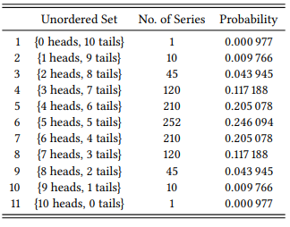
The basic idea behind statistical hypothesis testing is simple: we calculate the probability of the result that we have observed. The lower this probability is, the less likely it is to have come about by chance and the more probable is it that we will be right if we reject the null hypothesis. For example, if we observed a series of ten heads and zero tails, we know that the likelihood that the deviation from the expected result of five heads and five tails is due to chance is 0.000977 (i.e. roughly a tenth of a percent). This tenth of a percent is also the probability that we are wrong if we reject the null hypothesis and claim that the coin is not behaving randomly (for example, that it is manipulated in some way).

If we observed one heads and nine tails, we would know that the likelihood that this deviation from the expected result is 0.009766 (i.e. almost one percent). Thus we might think that, again, if we reject the null hypothesis, this is the probability that we are wrong. However, we must add to this the probability of getting ten heads and zero tails. The reason for this is that if we accept a result of 1:9 as evidence for a non-random distribution, we would also accept the even more extreme result of 0:10. So the probability that we are wrong in rejecting the null hypothesis is 0.000977 + 0.009766 = 0.010743. In other words: the probability that we are wrong in rejecting the null hypothesis is always the probability of the observed result plus the probabilities of all results that deviate from the null hypothesis even further in the direction of the observed frequency. This is called the probability of error (or simply p-value) in statistics.

It must be mentioned at this point that some researchers (especially opponents of null-hypothesis statistical significance testing) disagree that p can be interpreted as the probability that we are wrong in rejecting the null hypothesis, raising enough of a controversy to force the American Statistical Association to take an official stand on the meaning of p:

Informally, a p-value is the probability under a specified statistical model that a statistical summary of the data (e.g., the sample mean difference between two compared groups) would be equal to or more extreme than its observed value. (Wasserstein & Lazar 2016: 131)

Although this is the informal version of their definition, it may be completely incomprehensible at first glance, but it is actually just a summary of the discussion above: the “specified statistical model” in our case is the null hypothesis, i.e., the hypothesis that our data have come about purely by chance. The p-value thus tells us how probable it is under this hypothesis that we would observe the result we have observed, or an even more extreme result.

It also tells us how likely we are wrong if we reject this null hypothesis: If our model (i.e. the null hypothesis) will occasionally produce our observed result (or a more extreme one), then we will be wrong in rejecting it at those occasions. The p-value tells us, how likely it is that we are dealing with such an occasion. Of course, it does not tell us how likely it is that the null hypothesis is actually true or false – we do not know this likelihood and we can never know it. Statistical hypotheses are no different in this respect from universal hypotheses. Even if we observe a result with a probability of one in a million, the null hypothesis could be true (as we might be dealing with this one-in-a-million event), and even if we observe a result with a probability of 999 999 in a million, the null hypothesis could be false (as our result could nevertheless have come about by chance). The p-value simply tells us how likely it is that our study – with all its potential faults, confounding variables, etc. – would produce the result we observe and thus how likely we are wrong on the basis of this study to reject the null hypothesis. This simply means that we should not start believing in our hypothesis until additional studies have rejected the null hypothesis – an individual study may lead us to wrongly reject the null hypothesis, but the more studies we conduct that allow us to reject the null hypothesis, the more justified we are in treating them as corroborating our research hypothesis.

By convention, probability of error of 0.05 (five percent) is considered to be the limit as far as acceptable risks are concerned in statistics – if p < 0.05 (i.e., if p is smaller than five percent), the result is said to be statistically significant (i.e., not due to chance), if it is larger, the result is said to be non-significant (i.e., likely due to chance). Table 6.2 shows additional levels of significance that are conventionally recognized.

Table 6.2: Interpretation of p-values

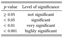
Obviously, these cut-off points are largely arbitrary (a point that is often criticized by opponents of null-hypothesis significance testing): it is strange to be confident in rejecting a null hypothesis if the probability of being wrong in doing so is five percent, but to refuse to reject it if the probability of being wrong is six percent (or, as two psychologists put it: “Surely, God loves the .06 nearly as much as the .05” (Rosnow & Rosenthal 1989: 1277)).

In real life, of course, researchers do not treat these cut-off points as absolute. Nobody would simply throw away a set of carefully collected data as soon as their calculations yielded a p-value of 0.06 or even 0.1. Some researchers actually report such results, calling p-values between 0.05 and 0.10 “marginally significant”, and although this is often frowned upon, there is nothing logically wrong with it. Even the majority of researchers who are unwilling to report such results would take them as an indicator that additional research might be in order (especially if there is a reasonable effect size, see further below).

They might re-check their operational definitions and the way they were applied, they might collect additional data in order to see whether a larger data set yields a lower probability of error, or they might replicate the study with a different data set. Note that this is perfectly legitimate, and completely in line with the research cycle sketched out in Section 3.3 – provided we retain all of our data. What we must not do, of course, is test different data sets until we find one that gives us a significant result, and then report just that result, ignoring all attempts that did not yield significant results. What we must also not do is collect an extremely large data set and then keep drawing samples from it until we happen to draw one that gives us a significant result. These practices are sometimes referred to as p-hacking, and they constitute a scientific fraud (imagine a a researcher who wants to corroborate their hypothesis that all swans are white and does so by simply ignoring all black swans they find).

Clearly, what probability of error one is willing to accept for any given study also depends on the nature of the study, the nature of the research design, and a general disposition to take or avoid risk. If mistakenly rejecting the null hypothesis were to endanger lives (for example, in a study of potential side-effects of a medical treatment), we might not be willing to accept a p-value of 0.05 or even 0.01.

Why would collecting additional data be a useful strategy, or, more generally speaking, why are corpus-linguists (and other scientists) often intent on making their samples as large as possible and/or feasible? Note that the probability of error depends not just on the proportion of the deviation, but also on the overall size of the sample. For example, if we observe a series of two heads and eight tails (i.e., twenty percent heads), the probability of error in rejecting the null hypothesis is 0.000977 + 0.009766 + 0.043945 = 0.054688. However, if we observe a series of four heads and sixteen tails (again, twenty percent heads), the probability of error would be roughly ten times lower, namely 0.005909. The reason is the following: There are 1 048 576 possible series of twenty coin flips. There is still only one way of getting one head and nineteen tails, so the probability of getting one head and nineteen tails is ¹/_1048576 = 0.0000009536743; however, there are already 20 ways of getting one tail and nineteen heads (so the probability is ²⁰/_1048576 = 0.000019), 190 ways of getting two heads and eighteen tails (p = ¹⁹⁰/_1048576 = 0.000181), 1140 ways of getting three heads and seventeen tails (p = ¹¹⁴⁰/_1048576 = 0.001087) and 4845 ways of getting four heads and sixteen tails (p = ⁴⁸⁴⁵/_1048576 = 0.004621). And adding up these probabilities gives us 0.005909.

Most research designs in any discipline are more complicated than coin flipping, which involves just a single variable with two values. However, it is theoretically possible to generalize the coin-flipping logic to any research design, i.e., calculate the probabilities of all possible outcomes and add up the probabilities of the observed outcome and all outcomes that deviate from the expected outcome even further in the same direction. Most of the time, however, this is only a theoretical possibility, as the computations quickly become too complex to be performed in a reasonable time frame even by supercomputers, let alone by a standard-issue home computer or manually.

Therefore, many statistical methods use a kind of mathematical detour: they derive from the data a single value whose probability distribution is known – a so-called test statistic. Instead of calculating the probability of our observed outcome directly, we can then assess its probability by comparing the test statistic against its known distribution. Mathematically, this involves identifying its position on the respective distribution and, as we did above, adding up the probability of this position and all positions deviating further from a random distribution. In practice, we just have to look up the test statistic in a chart that will give us the corresponding probability of error (or p-value, as we will call it from now on).

In the following three sections, I will introduce three widely-used tests involving test statistics for the three types of data discussed in the previous section: the chi-square (X ² ) test for nominal data, the Wilcoxon-Mann-Whitney test (also known as Mann-Whitney U test or Wilcoxon rank sum test) for ordinal data, and Welch’s t-test for cardinal data. I will also briefly discuss extensions of the X ² test for more complex research designs, including those involving more than two variables.

Given the vast range of corpus-linguistic research designs, these three tests will not always be the ideal choice. In many cases, there are more sophisticated statistical procedures which are better suited to the task at hand, be it for theoretical (mathematical or linguistic) or for practical reasons. However, the statistical tests introduced here have some advantages that make them ideal procedures for an initial statistical evaluation of results. For example, they are easy to perform: we don’t need more than a paper and a pencil, or a calculator, if we want to speed up things, and they are also included as standard functions in widely-used spreadsheet applications. They are also relatively robust in situations where we should not really use them (a point I will return to below).

They are also ideal procedures for introducing statistics to novices. Again, they are easy to perform and do not require statistical software packages that are typically expensive and/or have a steep learning curve. They are also relatively transparent with respect to their underlying logic and the steps required to perform them. Thus, my purpose in introducing them in some detail here is at least as much to introduce the logic and the challenges of statistical analysis, as it is to provide basic tools for actual research.

I will not introduce the mathematical underpinnings of these tests, and I will mention alternative and/or more advanced procedures only in passing – this includes, at least for now, research designs where neither variable is nominal. In these cases, correlation tests are used, such as Pearson’s product-moment correlations (if are dealing with two cardinal variables) and Spearman’s rank correlation coefficient or the Kendall tau rank correlation coefficient (if one or both of our variables are ordinal).

I will not, in other words, do much more than scratch the surface of the vast discipline of statistics. In the Study Notes to this chapter, there are a number of suggestions for further reading that are useful for anyone interested in a deeper understanding of the issues introduced here, and obligatory for anyone serious about using statistical methods in their own research. While I will not be making reference to any statistical software applications, such applications are necessary for serious quantitative research; again, the Study Notes contain useful suggestions where to look.

² You may remember having heard of Pascal’s triangle, which, among more sophisticated things, lets us calculate the number of different ways in which we can get a particular combination of heads and tails for a given number of coin flips: the third column of Table 6.1 corresponds to line 11 of this triangle. If you don’t remember, no worries, we will not need it.