6.3: Nominal data- The chi-square test

As mentioned in the preceding chapter, nominal data (or data that are best treated like nominal data) are the type of data most frequently encountered in corpus linguistics. I will therefore treat them in slightly more detail than the other two types, introducing different versions and (in the next chapter) extensions of the most widely used statistical test for nominal data, the chi-square (χ²) test. This test in all its variants is extremely flexible; it is thus more useful across different research designs than many of the more specific and more sophisticated procedures (much like a Swiss army knife is an excellent all-purpose tool despite the fact that there is usually a better tool dedicated to a specific task at hand).

Despite its flexibility, there are two requirements that must be met in order for the χ² test to be applicable: first, no intersection of variables must have a frequency of zero in the data, and second, no more than twenty-five percent of the intersections must have frequencies lower than five. When these conditions are not met, an alternative test must be used instead (or we need to collect additional data).

6.3.1 Two-by-two designs

Let us begin with a two-by-two design and return to the case of discourse-old and discourse-new modifiers in the two English possessive constructions. Here is the research hypothesis again, paraphrased from (9) and (11) in Chapter 5:

(3) H1 : There is a relationship between DISCOURSE STATUS and TYPE OF POSSESSIVE such that the S -POSSESSIVE is preferred when the modifier is DISCOURSE-OLD, the OF -POSSESSIVE is preferred when the modifier is DISCOURSE-NEW.

Prediction: There will be more cases of the S -POSSESSIVE with DISCOURSE-OLD modifiers than with discourse-new modifiers, and more cases of the OF -POSSESSIVE with discourse-new modifiers than with DISCOURSE-OLD modifiers.

The corresponding null hypothesis is stated in (4):

(4) H0 : There is no relationship between DISCOURSE STATUS and TYPE OF POSSESSIVE.

Prediction: Discourse-old and discourse-new modifiers will be distributed randomly across the two Possessive constructions.

We already reported the observed and expected frequencies in Table 5.4, but let us repeat them here as Table 6.3 for convenience in a slightly simplified form that we will be using from now on, with the expected frequencies shown in parentheses below the observed ones.

Table 6.3: Observed and expected frequencies of old and new modifiers in the s - and the of -possessive (= Table 5.4)

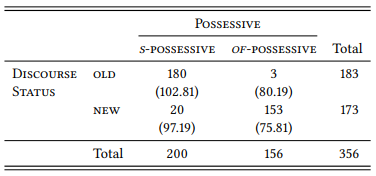
In order to test our research hypothesis, we must show that the observed frequencies differ from the null hypothesis in the direction of our prediction. We already saw in Chapter 5 that this is the case: The null hypothesis predicts the expected frequencies, but there are more cases of s -possessives with old modifiers and of -possessives with new modifiers than expected. Next, we must apply the coin-flip logic and ask the question: “Given the sample size, how surprising is the difference between the expected frequencies (i.e., a perfectly random distribution) and the observed frequencies (i.e., the distribution we actually find in our data)?”

As mentioned above, the conceptually simplest way of doing this would be to compute all possible ways in which the marginal frequencies (the sums of the columns and rows) could be distributed across the four cells of our table and then check what proportion of these tables deviates from a perfectly random distribution at least as much as the table we have actually observed. For two-by-two tables, there is, in fact, a test that does this, the exact test (also called Fisher’s exact test or, occasionally, Fisher-Yates exact test), and where the conditions for using the χ2 test are not met, we should use it. But, as mentioned above, this test is difficult to perform without statistical software, and it is not available for tables larger than 2-by-2 anyway, so instead we will derive the χ2 test statistic from the table.

First, we need to assess the magnitude of the differences between observed and expected frequencies. The simplest way of doing this would be to subtract the expected differences from the observed ones, giving us numbers that show for each cell the size of the deviation as well as its direction (i.e., are the observed frequencies higher or lower than the expected ones). For example, the values for Table 6.3 would be 77.19 for cell C11 (S -POSSESSIVE ∩ OLD), −77.19 for C21 (OF -POSSESSIVE ∩ OLD), −77.19 for C12 (S -POSSESSIVE ∩ NEW) and 77.19 for C22 (OF -POSSESSIVE ∩ NEW)

However, we want to derive a single measure from the table, so we need a measure of the overall deviation of the observed frequencies from the expected, not just a measure for the individual intersections. Obviously, adding up the differences of all intersections does not give us such a measure, as it would always be zero (since the marginal frequencies are fixed, any positive deviance in one cell will have a corresponding negative deviance in its neighboring cells). Second, subtracting the observed from the expected frequencies gives us the same number for each cell, when it is obvious that the actual magnitude of the deviation depends on the expected frequency. For example, a deviation of 77.19 is more substantial if the expected frequency is 75.81 than if the expected frequency is 102.81. In the first case, the observed frequency is more than a hundred percent higher than expected, in the second case, it is only 75 percent higher.

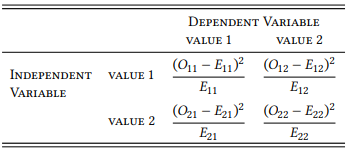
The first problem is solved by squaring the differences. This converts all deviations into positive numbers, and thus their sum will no longer be zero, and it has the additional effect of weighing larger deviations more strongly than smaller ones. The second problem is solved by dividing the squared difference by the expected frequencies. This will ensure that a deviation of a particular size will be weighed more heavily for a small expected frequency than for a large expected frequency. The values arrived at in this way are referred to as the cell components of χ² (or simply χ² components); the formulas for calculating the cell components in this way are shown in Table 6.4.

Table 6.4: Calculating χ² components for individual cells

If we apply this procedure to Table 6.3, we get the components shown in Table 6.5.

Table 6.5: χ² components for Table 6.3

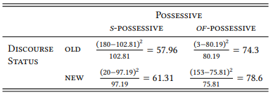
The degree of deviance from the expected frequencies for the entire table can then be calculated by adding up the χ² components. For Table 7.3, the χ² value (χ²) is 272.16. This value can now be used to determine the probability of error by checking it against a table like that in Section 14.1 in the Statistical Tables at the end of this book.

Before we can do so, there is a final technical point to make. Note that the degree of variation in a given table that is expected to occur by chance depends quite heavily on the size of the table. The bigger the table, the higher the number of cells that can vary independently of other cells without changing the marginal sums (i.e., without changing the overall distribution). The number of such cells that a table contains is referred to as the number of degrees of freedom of the table. In the case of a two-by-two table, there is just one such cell: if we change any single cell, we must automatically adjust the other three cells in order to keep the marginal sums constant. Thus, a two-by-two table has one degree of freedom.

The general formula for determining the degrees of freedom of a table is the following, where N_rows is the number of rows and N_column is the number of columns:

(5) df = (N_rows − 1) × (N_columns − 1)

Significance levels of χ² values differ depending on how many degrees of freedom a table has, so we always need to determine the degrees of freedom before we can determine the p-value. Turning to the table of χ² values in Section 14.1, we first find the row for one degree of freedom (this is the first row); we then check whether our χ² -value is larger than that required for the level of significance that we are after. In our case, the value of 272.16 is much higher than the χ² value required for a significance level of 0.001 at one degree of freedom, which is 10.83. Thus, we can say that the differences in Table 6.3 are statistically highly significant. The results of a χ² test are conventionally reported in the following format:

(6) Format for reporting the results of a χ² test (χ² = [chi-square value], df = [deg. of freedom], p < (or >) [sig. level])

In the present case, the analysis might be summarized along the following lines: “This study has shown that s -possessives are preferred when the modifier is discourse-old while of -possessives are preferred when the modifier is discourse-new. The differences between the constructions are highly significant (χ² = 272.16, df = 1, p < 0.001)”.

A potential danger to this way of formulating the results is the meaning of the word significant. In statistical terminology, this word simply means that the results obtained in a study based on one particular sample are unlikely to be due to chance and can therefore be generalized, with some degree of certainty, to the entire population. In contrast, in every-day usage the word means something along the lines of ‘having an important effect or influence’ (LDCE, s.v. significant). Because of this every-day use, it is easy to equate statistical significance with theoretical importance. However, there are at least three reasons why this equation must be avoided.

First, and perhaps most obviously, statistical significance has nothing to do with the validity of the operational definitions used in our research design. In our case, this validity is reasonably high, provided that we limit our conclusions to written English. As a related point, statistical significance has nothing to do with the quality of our data. If we have chosen unrepresentative data or if we have extracted or annotated our data sloppily, the statistical significance of the results is meaningless.

Second, statistical significance has nothing to do with theoretical relevance. Put simply, if we have no theoretical model in which the results can be interpreted meaningfully, statistical significance does not add to our understanding of the object of research. If, for example, we had shown that the preference for the two possessives differed significantly depending on the font in which a modifier is printed, rather than on the discourse status of the modifier, there is not much that we conclude from our findings.³

Third, and perhaps least obviously but most importantly, statistical significance does not actually tell us anything about the importance of the relationship we have observed. A relationship may be highly significant (i.e., generalizable with a high degree of certainty) and still be extremely weak. Put differently, statistical significance is not typically an indicator of the strength of the association.⁴

To solve the last problem, we can calculate a so-called measure of effect size, which, as its name suggests, indicates the size of the effect that our independent variable has on the dependent variable. For two-by-two contingency tables with categorical data, there is a widely-used measure referred to as ϕ (phi) that is calculated as follows:

(7)

In our example, this formula gives us

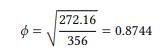
The ϕ -value is a so-called correlation coefficient, whose interpretation can be very subtle (especially when it comes to comparing two or more of them), but we will content ourselves with two relatively simple ways of interpreting them.

First, there are generally agreed-upon verbal descriptions for different ranges that the value of a correlation coefficient may have (similarly to the verbal descriptions of p -values discussed above. These descriptions are shown in Table 6.6.

Table 6.6: Conventional interpretation of correlation coefficients

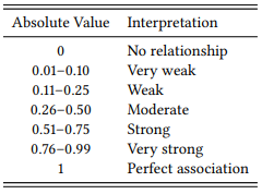
Our ϕ -value of 0.8744 falls into the very strong category, which is unusual in uncontrolled observational research, and which suggests that DISCOURSE STATUS is indeed a very important factor in the choice of POSSESSIVE constructions in English.

Exactly how much of the variance in the use of the two possessives is accounted for by the discourse status of the modifier can be determined by looking at the square of the ϕ coefficient: the square of a correlation coefficient generally tells us what proportion of the distribution of the dependent variable we can account for on the basis of the independent variable (or, more generally, what proportion of the variance our design has captured). In our case, ϕ ² = (0.8744 × 0.8744) = 0.7645. In other words, the variable DISCOURSE STATUS explains roughly three quarters of the variance in the use of the POSSESSIVE constructions – if, that is, our operational definition actually captures the discourse status of the modifier, and nothing else. A more precise way of reporting the results from our study would be something like the following “This study has shown a strong and statistically highly significant influence of DISCOURSE STATUS on the choice of possessive construction: s -possessives are preferred when the modifier is discourse-old (defined in this study as being realized by a pronoun) while of -possessives are preferred when the modifier is discourse-new (defined in this study as being realized by a lexical NP) (χ² = 272.16, df = 1, p < 0.001, ϕ ² = 0.7645)”.

Unfortunately, studies in corpus linguistics (and in the social sciences in general) often fail to report effect sizes, but we can usually calculate them from the data provided, and one should make a habit of doing so. Many effects reported in the literature are actually somewhat weaker than the significance levels might lead us to believe.

6.3.2 One-by-n designs

In the vast majority of corpus linguistic research issues, we will be dealing with designs that are at least bivariate (i.e., that involve the intersection of at least two variables), like the one discussed in the preceding section. However, once in a while we may need to test a univariate distribution for significance (i.e., a distribution of values of a single variable regardless of any specific condition). We may, for instance, have annotated an entire corpus for a particular speaker variable (such as sex), and we may now want to know whether the corpus is actually balanced with respect to this variable.

Consider the following example: the spoken part of the BNC contains language produced by 1317 female speakers and 2311 male speakers (as well as 1494 speakers whose sex is unknown, which we will ignore here). In order to determine whether the BNC can be considered a balanced corpus with respect to SPEAKER SEX, we can compare this observed distribution of speakers to the expected one more or less exactly in the way described in the previous sections except that we have two alternative ways of calculating the expected frequencies.

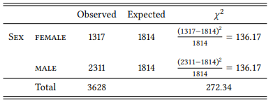
First, we could simply take the total number of elements and divide it by the number of categories (values), on the assumption that “random” distribution means that every category should occur with the same frequency. In this case, the expected number of MALE and FEMALE speakers would be [Total Number of Speakers / Sex Categories], i.e. ³⁶²⁸/₂ = 1814. We can now calculate the X ² components just as we did in the preceding sections, using the formula ((O − E)² )/E. Table 6.7 shows the results.

Adding up the components gives us a χ² value of 272.34. A one-by-two table has one degree of freedom (if we vary one cell, we have to adjust the other one automatically to keep the marginal sum constant). Checking the appropriate row in the table in Section 14.1, we can see that this value is much higher than the 10.83 required for a significance level of 0.01. Thus, we can say that “the BNC corpus contains a significantly higher proportion of male speakers than expected by chance (χ² = 272.34, df = 1, p < 0.001)” – in other words, the corpus is not balanced well with respect to the variable Speaker Sex (note that since this is a test of proportions rather than correlations, we cannot calculate a phi value here).

Table 6.7: Observed and expected frequencies of Speaker Sex in the BNC (based on the assumption of equal proportions)

The second way of deriving expected frequencies for a univariate distribution is from prior knowledge concerning the distribution of the values in general. In our case, we could find out the proportion of men and women in the relevant population and then derive the expected frequencies for our table by assuming that they follow this proportion. The relevant population in this case is that of the United Kingdom between 1991 and 1994, when the BNC was assembled. According to the World Bank, the women made up 51.4 percent and men 48.6 percent of the total population at that time, so the expected frequencies of male and female speakers in the corpus are as shown in Table 6.8.

Table 6.8: Observed and expected frequencies of Speaker Sex in the BNC (based on the proportions in the general population)

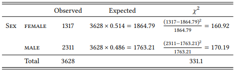
Clearly, the empirical distribution in this case closely resembles our hypothesized equal distribution, and thus the results are very similar – since there are slightly more women than men in the population, their underrepresentation in the corpus is even more significant.

Incidentally, the BNC not only contains speech by more male speakers than female speakers, it also includes more speech by male than by female speakers: men contribute 5 654 348 words, women contribute 3 825 804. I will leave it as an exercise to the reader to determine whether and in what direction these frequencies differ from what would be expected either under an assumption of equal proportions or given the proportion of female and male speakers in the corpus.

In the case of speaker sex it does not make much of a difference how we derive the expected frequencies, as men and women make up roughly half of the population each. For variables where such an even distribution of values does not exist, the differences between these two procedures can be quite drastic. As an example, consider Table 6.9, which lists the observed distribution of the speakers in the spoken part of the BNC across age groups (excluding speakers whose age is not recorded), together with the expected frequencies on the assumption of equal proportions, and the expected frequencies based on the distribution of speakers across age groups in the real world. The distribution of age groups in the population of the UK between 1991 and 1994 is taken from the website of the Office for National Statistics, averaged across the four years and cumulated to correspond to the age groups recorded in the BNC.

Table 6.9: Observed and expected frequencies of Speaker Age in the BNC

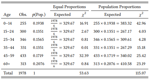
Adding up the χ² components gives us an overall χ² value of 53.63 in the first case and 115.07 in the second case. For univariate tables, df = (Number of Values – 1), so Table 6.9 has four degrees of freedom (we can vary four cells independently and then simply adjust the fifth to keep the marginal sum constant). The required χ² value for a 0.001-level of significance at four degrees of freedom is 18.47: clearly, whichever way we calculate the expected frequencies, the differences between observed and expected are highly significant. However, the distribution of age groups in the corpus is much closer to the assumption of equal proportions than to the actual proportions in the population; also, the conclusions we will draw concerning the over- or underrepresentation of individual categories will be very different. In the first case, for example, we might be led to believe that the age group 34–44 is fairly represented while the age group 15–24 is underrepresented. In the second case, we see that in fact both age groups are overrepresented. In this case, there is a clear argument for using empirically derived expected frequencies: the categories differ in terms of the age span each of them covers, so even if we thought that the distribution of ages in the population is homogeneous, we would not expect all categories to have the same size.

The exact alternative to the univariate χ² test with a two-level variable is the binomial test, which we used (without calling it that), in our coin-flip example in Section 6.2 above and which is included as a predefined function in many major spreadsheet applications and in R; for one-by-n tables, there is a multinomial test also available in R and other statistics packages.

³ This problem cannot be dismissed as lightly as this example may suggest: it points to a fundamental difficulty in doing science. Note that if we did find that the font has an influence on the choice of possessive, we would most likely dismiss this finding as a random fluke despite its statistical significance. And we may well be right, since even a level of significance of p < 0.001 does not preclude the possibility that the observed frequencies are due to chance. In contrast, an influence of the discourse status of the modifier makes sense because discourse status has been shown to have effects in many areas of grammar, and thus we are unlikely to question such an influence. In other words, our judgment of what is and is not plausible will influence our interpretation of our empirical results even if they are statistically significant. Alternatively, we could take every result seriously and look for a possible explanation, which will then typically require further investigation. For example, we might hypothesize that there is a relationship between font and level of formality, and the latter has been shown to have an influence on the choice of possessive constructions (Jucker 1993).

⁴ This statement must be qualified to a certain degree: given the right research design, statistical significance may actually be a very reasonable indicator of association strength (cf. e.g. Stefanowitsch & Gries 2003, Gries & Stefanowitsch 2004 for discussion). However, in most contexts we are well advised to keep statistical significance and association strength conceptually separate.