7.1: Collocates

The (orthographic) word plays a central role in corpus linguistics. As suggested in Chapter 4, this is in no small part due to the fact that all corpora, whatever additional annotations may have been added, consist of orthographically represented language. This makes it easy to retrieve word forms. Every concordancing program offers the possibility to search for a string of characters – in fact, some are limited to this kind of query.

However, the focus on words is also due to the fact that the results of corpus linguistic research quickly showed that words (individually and in groups) are more interesting and show a more complex behavior than traditional, grammar-focused theories of language assumed. An area in which this is very obvious, and which has therefore become one of the most heavily researched areas in corpus linguistics, is the way in which words combine to form so-called collocations.

This chapter is dedicated entirely to the discussion of collocation. At first, this will seem like a somewhat abrupt shift from the topics and phenomena we have discussed so far – it may not even be immediately obvious how they fit into the definition of corpus linguistics as “the investigation of linguistic research questions that have been framed in terms of the conditional distribution of linguistic phenomena in a linguistic corpus”, which was presented at the end of Chapter 2. However, a closer look will show that studying the co-occurrence of words and/ or word forms is simply a special case of precisely this kind of research program.

7.1 Collocates

Trivially, texts are not random sequences of words. There are several factors influencing the likelihood of two (or more) words occurring next to each other.

First, the co-occurrence of words in a sequence is restricted by grammatical considerations. For example, a definite article cannot be followed by another definite article or a verb, but only by a noun, by an adjective modifying a noun, by an adverb modifying such an adjective or by a post-determiner. Likewise, a transitive verb requires a direct object in the form of a noun phrase, so – barring cases where the direct object is pre- or post-posed – it will be followed by a word that can occur at the beginning of a noun phrase (such as a pronoun, a determiner, an adjective or a noun).

Second, the co-occurrence of words is restricted by semantic considerations. For example, the transitive verb drink requires a direct object referring to a liquid, so it is probable that it will be followed by words like water, beer, coffee, poison, etc., and improbable that it will be followed by words like bread, guitar, stone, democracy, etc. Such restrictions are treated as a grammatical property of words (called selection restrictions) in some theories, but they may also be an expression of our world knowledge concerning the activity of drinking.

Finally, and related to the issue of world knowledge, the co-occurrence of words is restricted by topical considerations. Words will occur in sequences that correspond to the contents we are attempting to express, so it is probable that co-occurring content words will come from the same discourse domain.

However, it has long been noted that words are not distributed randomly even within the confines of grammar, lexical semantics, world knowledge, and communicative intent. Instead, a given word will have affinities to some words, and disaffinities to others, which we could not predict given a set of grammatical rules, a dictionary and a thought that needs to be expressed. One of the first principled discussions of this phenomenon is found in Firth (1957). Using the example of the word ass (in the sense of ‘donkey’), he discusses the way in which what he calls habitual collocations contribute to the meaning of words:

One of the meanings of ass is its habitual collocation with an immediately preceding you silly, and with other phrases of address or of personal reference. ... There are only limited possibilities of collocation with preceding adjectives, among which the commonest are silly, obstinate, stupid, awful, occasionally egregious. Young is much more frequently found than old. (Firth 1957: 194f)

Note that Firth, although writing well before the advent of corpus linguistics, refers explicitly to frequency as a characteristic of collocations. The possibility of using frequency as part of the definition of collocates, and thus as a way of identifying them, was quickly taken up. Halliday (1961) provides what is probably the first strictly quantitative definition (cf. also Church & Hanks (1990) for a more recent comprehensive quantitative discussion):

Collocation is the syntagmatic association of lexical items, quantifiable, textually, as the probability that there will occur, at n removes (a distance of n lexical items) from an item x, the items a, b, c... Any given item thus enters into a range of collocation, the items with which it is collocated being ranged from more to less probable... (Halliday 1961: 276)

7.1.1 Collocation as a quantitative phenomenon

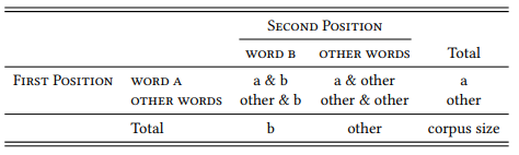
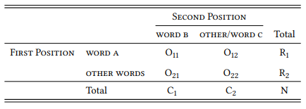
Essentially, then, collocation is just a special case of the quantitative corpus linguistic research design adopted in this book: to ask whether two words form a collocation (or: are collocates of each other) is to ask whether one of these words occurs in a given position more frequently than expected by chance under the condition that the other word occurs in a structurally or sequentially related position. In other words, we can decide whether two words a and b can be regarded as collocates on the basis of a contingency table like that in Table 7.1. The FIRST POSITION in the sequence is treated as the dependent variable, with two values: the word we are interested in (here: WORD A), and all OTHER words. The SECOND POSITION is treated as the independent variable, again, with two values: the word we are interested in (here: WORD B), and all OTHER words (of course, it does not matter which word we treat as the dependent and which as the independent variable, unless our research design suggests a particular reason).¹

Table 7.1: Collocation

On the basis of such a table, we can determine the collocation status of a given word pair. For example, we can ask whether Firth was right with respect to the claim that silly ass is a collocation. The necessary data are shown in Table 7.2: As discussed above, the dependent variable is the FIRST POSITION in the sequence, with the values SILLY and ¬SILLY (i.e., all words that are not ass); the independent variable is the SECOND POSITION in the sequence, with the values ASS and ¬ASS.

Table 7.2: Co-occurrence of silly and ass in the BNC

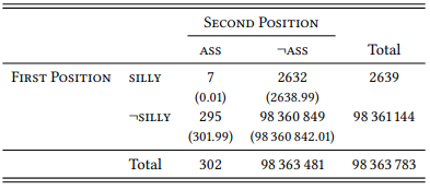
The combination silly ass is very rare in English, occurring just seven times in the 98 363 783 word BNC, but the expected frequencies in Table 7.2 show that this is vastly more frequent than should be the case if the words co-occurred randomly – in the latter case, the combination should have occurred just 0.01 times (i.e., not at all). The difference between the observed and the expected frequencies is highly significant (χ² = 6033.8, df = 1, p < 0.001). Note that we are using the χ² test here because we are already familiar with it. However, this is not the most useful test for the purpose of identifying collocations, so we will discuss better options below.

Generally speaking, the goal of a quantitative collocation analysis is to identify, for a given word, those other words that are characteristic for its context of usage. Tables 7.1 and 7.2 present the most straightforward way of doing so: we simply compare the frequency with which two words co-occur to the frequencies with which they occur in the corpus in general. In other words, the two conditions across which we are investigating the distribution of a word are “next to a given other word” and “everywhere else”. This means that the corpus itself functions as a kind of neutral control condition, albeit a somewhat indiscriminate one: comparing the frequency of a word next to some other word to its frequency in the entire rest of the corpus is a bit like comparing an experimental group of subjects that have been given a particular treatment to a control group consisting of all other people who happen to live in the same city.

Often, we will be interested in the distribution of a word across two specific conditions – in the case of collocation, the distribution across the immediate contexts of two semantically related words. It may be more insightful to compare adjectives occurring next to ass with those occurring next to the rough synonym donkey or the superordinate term animal. Obviously, the fact that silly occurs more frequently with ass than with donkey or animal is more interesting than the fact that silly occurs more frequently with ass than with stone or democracy. Likewise, the fact that silly occurs with ass more frequently than childish is more interesting than the fact that silly occurs with ass more frequently than precious or parliamentary.

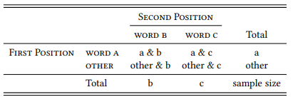
In such cases, we can modify Table 7.1 as shown in Table 7.3 to identify the collocates that differ significantly between two words. There is no established term for such collocates, so we we will call them differential collocates here² (the method is based on Church et al. 1991).

Table 7.3: Identifying differential collocates

Since the collocation silly ass and the word ass in general are so infrequent in the BNC, let us use a different noun to demonstrate the usefulness of this method, the word game. We can speak of silly game(s) or childish game(s), but we may feel that the latter is more typical than the former. The relevant lemma frequencies to put this feeling to the test are shown in Table 7.4.

Table 7.4: Childish game vs. silly game (lemmas) in the BNC

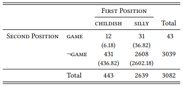
The sequences childish game(s) and silly game(s) both occur in the BNC. Both combinations taken individually are significantly more frequent than expected (you may check this yourself using the frequencies from Table 7.4, the total lemma frequency of game in the BNC (20 627), and the total number of words in the BNC given in Table 7.2 above). The lemma sequence silly game is more frequent, which might lead us to assume that it is the stronger collocation. However, the direct comparison shows that this is due to the fact that silly is more frequent in general than childish, making the combination silly game more probable than the combination childish game even if the three words were distributed randomly. The difference between the observed and the expected frequencies suggests that childish is more strongly associated with game(s) than silly. The difference is significant (χ² = 6.49, df = 1, p < 0.05).

Researchers differ with respect to what types of co-occurrence they focus on when identifying collocations. Some treat co-occurrence as a purely sequential phenomenon defining collocates as words that co-occur more frequently than expected within a given span. Some researchers require a span of 1 (i.e., the words must occur directly next to each other), but many allow larger spans (five words being a relatively typical span size).

Other researchers treat co-occurrence as a structural phenomenon, i.e., they define collocates as words that co-occur more frequently than expected in two related positions in a particular grammatical structure, for example, the adjective and noun positions in noun phrases of the form [Det Adj N] or the verb and noun position in transitive verb phrases of the form [V [_NP (Det) (Adj) N]].³ However, instead of limiting the definition to one of these possibilities, it seems more plausible to define the term appropriately in the context of a specific research question. In the examples above, we used a purely sequential definition that simply required words to occur next to each other, paying no attention to their word-class or structural relationship; given that we were looking at adjective-noun combinations, it would certainly have been reasonable to restrict our search parameters to adjectives modifying the noun ass, regardless of whether other adjectives intervened, for example in expressions like silly old ass, which our query would have missed if they occurred in the BNC (they do not).

It should have become clear that the designs in Tables 7.1 and 7.3 are essentially variants of the general research design introduced in previous chapters and used as the foundation of defining corpus linguistics: it has two variables, POSITION 1 and POSITION 2, both of which have two values, namely WORD X VS. OTHER WORDS (or, in the case of differential collocates, WORD X VS. WORD Y). The aim is to determine whether the value WORD A is more frequent for POSITION 1 under the condition that WORD B occurs in POSITION 2 than under the condition that other words (or a particular other word) occur in POSITION 2.

7.1.2 Methodological issues in collocation research

We may occasionally be interested in an individual pair of collocates, such as silly ass, or in a small set of such pairs, such as all adjective-noun pairs with ass as the noun. However, it is much more likely that we will be interested in large sets of collocate pairs, such as all adjective-noun pairs or even all word pairs in a given corpus. This has a number of methodological consequences concerning the practicability, the statistical evaluation and the epistemological status of collocation research.

a. Practicability. In practical terms, the analysis of large numbers of potential collocations requires creating a large number of contingency tables and subjecting them to the χ² test or some other appropriate statistical test. This becomes implausibly time-consuming very quickly and thus needs to be automated in some way.

There are concordancing programs that offer some built-in statistical tests, but they typically restrict our options quite severely, both in terms of the tests they allow us to perform and in terms of the data on which the tests are performed. Anyone who decides to become involved in collocation research (or some of the large-scale lexical research areas described in the next chapter), should get acquainted at least with the simple options of automatizing statistical testing offered by spreadsheet applications. Better yet, they should invest a few weeks (or, in the worst case, months) to learn a scripting language like Perl, Python or R (the latter being a combination of statistical software and programming environment that is ideal for almost any task that we are likely to come across as corpus linguists).

b. Statistical evaluation. In statistical terms, the analysis of large numbers of potential collocations requires us to keep in mind that we are now performing multiple significance tests on the same set of data. This means that we must adjust our significance levels. Think back to the example of coin-flipping: the probability of getting a series of one head and nine tails is 0.009765. If we flip a coin ten times and get this result, we could thus reject the null hypothesis with a probability of error of 0.010744, i.e., around 1 percent (because we would have to add the probability of getting ten tails, 0.000976). This is well below the level required to claim statistical significance. However, if we perform one hundred series of ten coin-flips and one of these series consists of one head and nine tails (or ten tails), we could not reject the null hypothesis with the same confidence, as a probability of 0.010744 means that we would expect one such series to occur by chance. This is not a problem as long as we do not accord this one result out of a hundred any special importance. However, if we were to identify a set of 100 collocations with p -values of 0.001 in a corpus, we are potentially treating all of them as important, even though it is very probable that at least one of them reached this level of significance by chance.

To avoid this, we have to correct our levels of significance when performing multiple tests on the same set of data. As discussed in Section 6.6.1 above, the simplest way to do this is the Bonferroni correction, which consists in dividing the conventionally agreed-upon significance levels by the number of tests we are performing. As noted in Section 6.6.1, this is an extremely conservative correction that might make it quite difficult for any given collocation to reach significance.

Of course, the question is how important the role of p -values is in a design where our main aim is to identify collocates and order them in terms of their collocation strength. I will turn to this point presently, but before I do so, let us discuss the third of the three consequences of large-scale testing for collocation, the methodological one.

c. Epistemological considerations. We have, up to this point, presented a very narrow view of the scientific process based (in a general way) on the Popperian research cycle where we formulate a research hypothesis and then test it (either directly, by looking for counterexamples, or, more commonly, by attempting to reject the corresponding null hypothesis). This is called the deductive method. However, as briefly discussed in Chapter 3, there is an alternative approach to scientific research that does not start with a hypothesis, but rather with general questions like “Do relationships exist between the constructs in my data?” and “If so, what are those relationships?”. The research then consists in applying statistical procedures to large amounts of data and examining the results for interesting patterns. As electronic storage and computing power have become cheaper and more widely accessible, this approach – the exploratory or inductive approach – has become increasingly popular in all branches of science, particularly the social sciences. It would be surprising if corpus linguistics was an exception, and indeed, it is not. Especially the area of collocational research is typically exploratory.

In principle, there is nothing wrong with exploratory research – on the contrary, it would be unreasonable not to make use of the large amounts of language data and the vast computing power that has become available and accessible over the last thirty years. In fact, it is sometimes difficult to imagine a plausible hypothesis for collocational research projects. What hypothesis would we formulate before identifying all collocations in the LOB or some specialized corpus (e.g., a corpus of business correspondence, a corpus of flight-control communication or a corpus of learner language)?⁴ Despite this, it is clear that the results of such a collocation analysis yield interesting data, both for practical purposes (building dictionaries or teaching materials for business English or aviation English, extracting terminology for the purpose of standardization, training natural-language processing systems) and for theoretical purposes (insights into the nature of situational language variation or even the nature of language in general).

But there is a danger, too: Most statistical procedures will produce some statistically significant result if we apply them to a large enough data set, and collocational methods certainly will. Unless we are interested exclusively in description, the crucial question is whether these results are meaningful. If we start with a hypothesis, we are restricted in our interpretation of the data by the need to relate our data to this hypothesis. If we do not start with a hypothesis, we can interpret our results without any restrictions, which, given the human propensity to see patterns everywhere, may lead to somewhat arbitrary post-hoc interpretations that could easily be changed, even reversed, if the results had been different and that therefore tell us very little about the phenomenon under investigation or language in general. Thus, it is probably a good idea to formulate at least some general expectations before doing a large-scale collocation analysis.

Even if we do start out with general expectations or even with a specific hypothesis, we will often discover additional facts about our phenomenon that go beyond what is relevant in the context of our original research question. For example, checking in the BNC Firth’s claim that the most frequent collocates of ass are silly, obstinate, stupid, awful and egregious and that young is “much more frequent” than old, we find that silly is indeed the most frequent adjectival collocate, but that obstinate, stupid and egregious do not occur at all, that awful occurs only once, and that young and old both occur twice. Instead, frequent adjectival collocates (ignoring second-placed wild, which exclusively refers to actual donkeys), are pompous and bad. Pompous does not really fit with the semantics that Firth’s adjectives suggest and could indicate that a semantic shift from ‘stupidity’ to ‘self-importance’ may have taken place between 1957 and 1991 (when the BNC was assembled).

This is, of course, a new hypothesis that can (and must) be investigated by comparing data from the 1950s and the 1990s. It has some initial plausibility in that the adjectives blithering, hypocritical, monocled and opinionated also co-occur with ass in the BNC but are not mentioned by Firth. However, it is crucial to treat this as a hypothesis rather than a result. The same goes for bad ass which suggests that the American sense of ass (‘bottom’) and/or the American adjective badass (which is often spelled as two separate words) may have begun to enter British English. In order to be tested, these ideas – and any ideas derived from an exploratory data analysis – have to be turned into testable hypotheses and the constructs involved have to be operationalized. Crucially, they must be tested on a new data set – if we were to circularly test them on the same data that they were derived from, we would obviously find them confirmed.

7.1.3 Effect sizes for collocations

As mentioned above, significance testing (while not without its uses) is not necessarily our primary concern when investigating collocations. Instead, researchers frequently need a way of assessing the strength of the association between two (or more) words, or, put differently, the effect size of their co-occurrence (recall from Chapter 6 that significance and effect size are not the same). A wide range of such association measures has been proposed and investigated. They are typically calculated on the basis of (some or all) the information contained in contingency tables like those in Tables 7.1 and 7.3 above.

Let us look at some of the most popular and/or most useful of these measures. I will represent the formulas with reference to the table in Table 7.5, i.e, O₁₁ means the observed frequency of the top left cell, E₁₁ its expected frequency, R₁ the first row total, C₂ the second column total, and so on. Note that second column would be labeled OTHER WORDS in the case of normal collocations, and WORD C in the case of differential collocations. The association measures can be applied to both kinds of design.

Table 7.5: A generic 2-by-2 table for collocation research

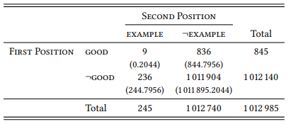
Now all we need is a good example to demonstrate the calculations. Let us use the adjective-noun sequence good example from the LOB corpus (but horse lovers need not fear, we will return to equine animals and their properties below).

Table 7.6: Co-occurrence of good and example in the LOB

Measures of collocation strength differ with respect to the data needed to calculate them, their computational intensiveness and, crucially, the quality of their results. In particular, many measures, notably the ones easy to calculate, have a problem with rare collocations, especially if the individual words of which they consist are also rare. After we have introduced the measures, we will therefore compare their performance with a particular focus on the way in which they deal (or fail to deal) with such rare events.

7.1.3.1 Chi-square

The first association measure is an old acquaintance: the chi-square statistic, which we used extensively in Chapter 6 and in Section 7.1.1 above. I will not demonstrate it again, but the chi-square value for Table 7.6 would be 378.95 (at 1 degree of freedom this means that p < 0.001, but we are not concerned with p -values here).

Recall that the chi-square test statistic is not an effect size, but that it needs to be divided by the table total to turn it into one. As long as we are deriving all our collocation data from the same corpus, this will not make a difference, since the table total will always be the same. However, this is not always the case. Where table sizes differ, we might consider using the phi value instead. I am not aware of any research using phi as an association measure, and in fact the chi-square statistic itself is not used widely either. This is because it has a serious problem: recall that it cannot be applied if more than 20 percent of the cells of the contingency table contain expected frequencies smaller than 5 (in the case of collocates, this means not even one out of the four cells of the 2-by-2 table). One reason for this is that it dramatically overestimates the effect size and significance of such events, and of rare events in general. Since collocations are often relatively rare events, this makes the chi-square statistic a bad choice as an association measure.

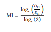
7.1.3.2 Mutual Information

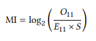
Mutual information is one of the oldest collocation measures, frequently used in computational linguistics and often implemented in collocation software. It is given in (1) in a version based on Church & Hanks (1990):⁵

(1)

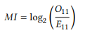
Applying the formula to our table, we get the following:

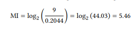
In our case, we are looking at cases where WORD A and WORD B occur directly next to each other, i.e., the span size is 1. When looking at a larger span (which is often done in collocation research), the probability of encountering a particular collocate increases, because there are more slots that it could potentially occur in. The MI statistic can be adjusted for larger span sizes as follows (where S is the span size):

(2)

The mutual information measure suffers from the same problem as the χ² statistic: it overestimates the importance of rare events. Since it is still fairly widespread in collocational research, we may nevertheless need it in situations where we want to compare our own data to the results of published studies. However, note that there are versions of the MI measure that will give different results, so we need to make sure we are using the same version as the study we are comparing our results to. But unless there is a pressing reason, we should not use mutual information at all.

7.1.3.3 The log-likelihood ratio test

The G value of the log-likelihood ratio test is one of the most popular – perhaps the most popular – association measure in collocational research, found in many of the central studies in the field and often implemented in collocation software. The following is a frequently found form (Read & Cressie 1988: 134):

(3)

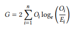
In order to calculate the G measure, we calculate for each cell the natural logarithm of the observed frequency divided by the expected frequency and multiply it by the observed frequency. We then add up the results for all four cells and multiply the result by two. Note that if the observed frequency of a given cell is zero, the expression ^O_i/_Ei will, of course, also be zero. Since the logarithm of zero is undefined, this would result in an error in the calculation. Thus, log(0) is simply defined as zero when applying the formula in (3).

Applying the formula in (3) to the data in Table 7.6, we get the following:

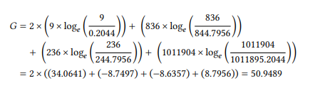
The G value has long been known to be more reliable than the χ² test when dealing with small samples and small expected frequencies (Read & Cressie 1988: 134ff). This led Dunning (1993) to propose it as an association measure specifically to avoid the overestimation of rare events that plagues the χ² test, mutual information and other measures.

7.1.3.4 Minimum Sensitivity

Minimum sensitivity was proposed by Pedersen (1998) as potentially useful measure especially for the identification of associations between content words:

(4)

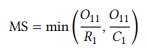
We simply divide the observed frequency of a collocation by the frequency of the first word (R₁) and of the second word (C₁) and use the smaller of the two as the association measure. For the data in Table 7.6, this gives us the following:

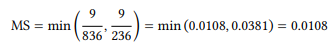
In addition to being extremely simple to calculate, it has the advantage of ranging from zero (words never occur together) to 1 (words always occur together); it was also argued by Wiechmann (2008) to correlate best with reading time data when applied to combinations of words and grammatical constructions (see Chapter 8). However, it also tends to overestimate the importance of rare collocations.

7.1.3.5 Fisher’s exact test

isher’s exact test was already mentioned in passing in Chapter 6 as an alternative to the χ² test that calculates the probability of error directly by adding up the probability of the observed distribution and all distributions that deviate from the null hypothesis further in the same direction. Pedersen (1996) suggests using this p -value as a measure of association because it does not make any assumptions about normality and is even better at dealing with rare events than G. Stefanowitsch & Gries (2003: 238–239) add that it has the advantage of taking into account both the magnitude of the deviation from the expected frequencies and the sample size.

There are some practical disadvantages to Fisher’s exact test. First, it is computationally expensive – it cannot be calculated manually, except for very small tables, because it involves computing factorials, which become very large very quickly. For completeness’ sake, here is (one version of) the formula:

(5)

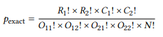
Obviously, it is not feasible to apply this formula directly to the data in Table 7.6, because we cannot realistically calculate the factorials for 236 or 836, let alone 1 011 904. But if we could, we would find that the p -value for Table 7.6 is 0.000000000001188.

Spreadsheet applications do not usually offer Fisher’s exact test, but all major statistics applications do. However, typically, the exact p -value is not reported beyond the limit of a certain number of decimal places. This means that there is often no way of ranking the most strongly associated collocates, because their p -values are smaller than this limit. For example, there are more than 100 collocates in the LOB corpus with a Fisher’s exact p -value that is smaller than the smallest value that a standard-issue computer chip is capable of calculating, and more than 5000 collocates that have ​​​​​​​p -values that are smaller than what the standard implementation of Fisher’s exact test in the statistical software package R will deliver. Since in research on collocations we often need to rank collocations in terms of their strength, this may become a problem.

7.1.3.6 A comparison of association measures

Let us see how the association measures compare using a data set of 20 potential collocations. Inspired by Firth’s silly ass, they are all combinations of adjectives with equine animals. Table 7.7 shows the combinations and their frequencies in the BNC sorted by their raw frequency of occurrence (adjectives and nouns are shown in small caps here to stress that they are values of the variables Word A and Word B, but I will generally show them in italics in the remainder of the book in line with linguistic tradition).

All combinations are perfectly normal, grammatical adjective-noun pairs, meaningful not only in the specific context of their actual occurrence. However, I have selected them in such a way that they differ with respect to their status as potential collocations (in the sense of typical combinations of words). Some are compounds or compound like combinations (rocking horse, Trojan horse, and, in specialist discourse, common zebra). Some are the kind of semi-idiomatic combinations that Firth had in mind (silly ass, pompous ass). Some are very conventional combinations of nouns with an adjective denoting a property specific to that noun (prancing horse, braying donkey, galloping horse – the first of these being a conventional way of referring to the Ferrari brand mark logo). Some only give the appearance of semi-idiomatic combinations (jumped-up jackass, actually an unconventional variant of jumped-up jack-in-office; dumb-fuck donkey, actually an extremely rare phrase that occurs only once in the documented history of English, namely in the book Trail of the Octopus: From Beirut to Lockerbie – Inside the DIA and that probably sounds like an idiom because of the alliteration and the semantic relationship to silly ass; and monocled ass, which brings to mind pompous ass but is actually not a very conventional combination). Finally, there are a number of fully compositional combinations that make sense but do not have any special status (caparisoned mule, new horse, old donkey, young zebra, large mule, female hinny, extinct quagga).

Table 7.7: Some collocates of the form [ADJ N_equine] (BNC)

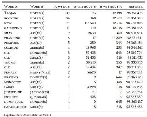
In addition, I have selected them to represent different types of frequency relations: some of them are (relatively) frequent, some of them very rare, for some of them the either the adjective or the noun is generally quite frequent, and for some of them neither of the two is frequent.

Table 7.8 shows the ranking of these twenty collocations by the five association measures discussed above. Simplifying somewhat, a good association measure should rank the conventionalized combinations highest (rocking horse, Trojan horse, silly ass, pompous ass, prancing horse, braying donkey, galloping horse), the distinctive sounding but non-conventionalized combinations somewhere in the middle (jumped-up jackass, dumb-fuck donkey, old ass, monocled ass) and the compositional combinations lowest (common zebra, jumped-up jackass, dumb-fuck donkey, old ass, monocled ass). Common zebra is difficult to predict – it is a conventionalized expression, but not in the general language.

Table 7.8: Comparison of selected association measures for collocates of the form [ADJ N_equine] (BNC)

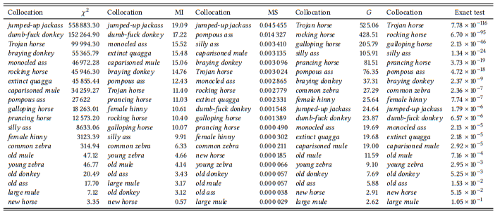
All association measures fare quite well, generally speaking, with respect to the compositional expressions – these tend to occur in the lower third of all lists. Where there are exceptions, the χ² statistic, mutual information and minimum sensitivity rank rare cases higher than they should (e.g. caparisoned mule, extinct quagga), while the G and the p -value of Fisher’s exact test rank frequent cases higher (e.g.galloping horse).

With respect to the non-compositional cases, χ² and mutual information are quite bad, overestimating rare combinations like jumped-up jackass, dumb-fuck donkey and monocled ass, while listing some of the clear cases of collocations much further down the list (silly ass, and, in the case of MI, rocking horse). Minimum sensitivity is much better, ranking most of the conventionalized cases in the top half of the list and the non-conventionalized ones further down (with the exception of jumped-up jackass, where both the individual words and their combination are very rare). The G and the Fisher p -value fare best (with no differences in their ranking of the expressions), listing the conventionalized cases at the top and the distinctive but non-conventionalized cases in the middle.

To demonstrate the problems that very rare events can cause (especially those where both the combination and each of the two words in isolation are very rare), imagine someone had used the phrase tomfool onager once in the BNC. Since neither the adjective tomfool (a synonym of silly) nor the noun onager (the name of the donkey sub-genus Equus hemionus, also known as Asiatic or Asian wild ass) occur in the BNC anywhere else, this would give us the distribution in Table 7.9.

Table 7.9: Fictive occurrence of tomfool onager in the BNC

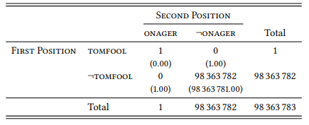
Applying the formulas discussed above to this table gives us a χ² value of 98 364 000, an MI value of 26.55 and a minimum sensitivity value of 1, placing this (hypothetical) one-off combination at the top of the respective rankings by a wide margin. Again, the log-likelihood ratio test and Fisher’s exact test are much better, putting in eighth place on both lists (G = 36.81, p_exact = 1.02 × 10⁻⁸ ).

Although the example is hypothetical, the problem is not. It uncovers a mathematical weakness of many commonly used association measures. From an empirical perspective, this would not necessarily be a problem, if cases like that in Table 7.9 were rare in linguistic corpora. However, they are not. The LOB corpus, for example, contains almost one thousand such cases, including some legitimate collocation candidates (like herbal brews, casus belli or sub-tropical climates), but mostly compositional combinations (ungraceful typography, turbaned headdress, songs-of-Britain medley), snippets of foreign languages (freie Blicke, l’arbre rouge, palomita blanca) and other things that are quite clearly not what we are looking for in collocation research. All of these will occur at the top of any collocate list created using statistics like χ² , mutual information and minimum sensitivity. In large corpora, which are impossible to check for orthographical errors and/or errors introduced by tokenization, this list will also include hundreds of such errors (whose frequency of occurrence is low precisely because they are errors).

To sum up, when doing collocational research, we should use the best association measures available. For the time being, this is the p value of Fisher’s exact test (if we have the means to calculate it), or G (if we don’t, or if we prefer using a widely-accepted association measure). We will use G through much of the remainder of this book whenever dealing with collocations or collocation-like phenomena.

¹ Note that we are using the corpus size as the table total – strictly speaking, we should be using the total number of two-word sequences (bigrams) in the corpus, which will be lower: The last word in each file of our corpus will not have a word following it, so we would have to subtract the last word of each file – i.e., the number of files in our corpus – from the total. This is unlikely to make much of a difference in most cases, but the shorter the texts in our corpus are, the larger the difference will be. For example, in a corpus of tweets, which, at the time of writing, are limited to 280 characters, it might be better to correct the total number of bigrams in the way described.

² Gries (2003b) and Gries & Stefanowitsch (2004) use the term distinctive collocate, which has been taken up by some authors; however, many other authors use the term distinctive collocate much more broadly to refer to characteristic collocates of a word.

³ Note that such word-class specific collocations are sometimes referred to as colligations, although the term colligation usually refers to the co-occurrence of a word in the context of particular word classes, which is not the same.

⁴ Of course we are making the implicit assumption that there will be collocates – in a sense, this is a hypothesis, since we could conceive of models of language that would not predict their existence (we might argue, for example, that at least some versions of generative grammar constitute such models). However, even if we accept this as a hypothesis, it is typically not the one we are interested in this kind of study.

⁵ A logarithm with a base b of a given number x is the power to which b must be raised to produce x, so, for example, log₁₀(2) = 0.30103, because 10^0.30103 = 2. Most calculators offer at the very least a choice between the natural logarithm, where the base is the number e (approx. 2.7183) and the common logarithm, where the base is the number 10; many calculators and all major spreadsheet programs offer logarithms with any base. In the formula in (1), we need the logarithm with base 2; if this is not available, we can use the natural logarithm and divide the result by the natural logarithm of 2: