7.2: Case studies
- Last updated
- Save as PDF
- Page ID
- 81929
\( \newcommand{\vecs}[1]{\overset { \scriptstyle \rightharpoonup} {\mathbf{#1}} } \)
\( \newcommand{\vecd}[1]{\overset{-\!-\!\rightharpoonup}{\vphantom{a}\smash {#1}}} \)
\( \newcommand{\id}{\mathrm{id}}\) \( \newcommand{\Span}{\mathrm{span}}\)
( \newcommand{\kernel}{\mathrm{null}\,}\) \( \newcommand{\range}{\mathrm{range}\,}\)
\( \newcommand{\RealPart}{\mathrm{Re}}\) \( \newcommand{\ImaginaryPart}{\mathrm{Im}}\)
\( \newcommand{\Argument}{\mathrm{Arg}}\) \( \newcommand{\norm}[1]{\| #1 \|}\)
\( \newcommand{\inner}[2]{\langle #1, #2 \rangle}\)
\( \newcommand{\Span}{\mathrm{span}}\)
\( \newcommand{\id}{\mathrm{id}}\)
\( \newcommand{\Span}{\mathrm{span}}\)
\( \newcommand{\kernel}{\mathrm{null}\,}\)
\( \newcommand{\range}{\mathrm{range}\,}\)
\( \newcommand{\RealPart}{\mathrm{Re}}\)
\( \newcommand{\ImaginaryPart}{\mathrm{Im}}\)
\( \newcommand{\Argument}{\mathrm{Arg}}\)
\( \newcommand{\norm}[1]{\| #1 \|}\)
\( \newcommand{\inner}[2]{\langle #1, #2 \rangle}\)
\( \newcommand{\Span}{\mathrm{span}}\) \( \newcommand{\AA}{\unicode[.8,0]{x212B}}\)
\( \newcommand{\vectorA}[1]{\vec{#1}} % arrow\)
\( \newcommand{\vectorAt}[1]{\vec{\text{#1}}} % arrow\)
\( \newcommand{\vectorB}[1]{\overset { \scriptstyle \rightharpoonup} {\mathbf{#1}} } \)
\( \newcommand{\vectorC}[1]{\textbf{#1}} \)
\( \newcommand{\vectorD}[1]{\overrightarrow{#1}} \)
\( \newcommand{\vectorDt}[1]{\overrightarrow{\text{#1}}} \)
\( \newcommand{\vectE}[1]{\overset{-\!-\!\rightharpoonup}{\vphantom{a}\smash{\mathbf {#1}}}} \)
\( \newcommand{\vecs}[1]{\overset { \scriptstyle \rightharpoonup} {\mathbf{#1}} } \)
\( \newcommand{\vecd}[1]{\overset{-\!-\!\rightharpoonup}{\vphantom{a}\smash {#1}}} \)
\(\newcommand{\avec}{\mathbf a}\) \(\newcommand{\bvec}{\mathbf b}\) \(\newcommand{\cvec}{\mathbf c}\) \(\newcommand{\dvec}{\mathbf d}\) \(\newcommand{\dtil}{\widetilde{\mathbf d}}\) \(\newcommand{\evec}{\mathbf e}\) \(\newcommand{\fvec}{\mathbf f}\) \(\newcommand{\nvec}{\mathbf n}\) \(\newcommand{\pvec}{\mathbf p}\) \(\newcommand{\qvec}{\mathbf q}\) \(\newcommand{\svec}{\mathbf s}\) \(\newcommand{\tvec}{\mathbf t}\) \(\newcommand{\uvec}{\mathbf u}\) \(\newcommand{\vvec}{\mathbf v}\) \(\newcommand{\wvec}{\mathbf w}\) \(\newcommand{\xvec}{\mathbf x}\) \(\newcommand{\yvec}{\mathbf y}\) \(\newcommand{\zvec}{\mathbf z}\) \(\newcommand{\rvec}{\mathbf r}\) \(\newcommand{\mvec}{\mathbf m}\) \(\newcommand{\zerovec}{\mathbf 0}\) \(\newcommand{\onevec}{\mathbf 1}\) \(\newcommand{\real}{\mathbb R}\) \(\newcommand{\twovec}[2]{\left[\begin{array}{r}#1 \\ #2 \end{array}\right]}\) \(\newcommand{\ctwovec}[2]{\left[\begin{array}{c}#1 \\ #2 \end{array}\right]}\) \(\newcommand{\threevec}[3]{\left[\begin{array}{r}#1 \\ #2 \\ #3 \end{array}\right]}\) \(\newcommand{\cthreevec}[3]{\left[\begin{array}{c}#1 \\ #2 \\ #3 \end{array}\right]}\) \(\newcommand{\fourvec}[4]{\left[\begin{array}{r}#1 \\ #2 \\ #3 \\ #4 \end{array}\right]}\) \(\newcommand{\cfourvec}[4]{\left[\begin{array}{c}#1 \\ #2 \\ #3 \\ #4 \end{array}\right]}\) \(\newcommand{\fivevec}[5]{\left[\begin{array}{r}#1 \\ #2 \\ #3 \\ #4 \\ #5 \\ \end{array}\right]}\) \(\newcommand{\cfivevec}[5]{\left[\begin{array}{c}#1 \\ #2 \\ #3 \\ #4 \\ #5 \\ \end{array}\right]}\) \(\newcommand{\mattwo}[4]{\left[\begin{array}{rr}#1 \amp #2 \\ #3 \amp #4 \\ \end{array}\right]}\) \(\newcommand{\laspan}[1]{\text{Span}\{#1\}}\) \(\newcommand{\bcal}{\cal B}\) \(\newcommand{\ccal}{\cal C}\) \(\newcommand{\scal}{\cal S}\) \(\newcommand{\wcal}{\cal W}\) \(\newcommand{\ecal}{\cal E}\) \(\newcommand{\coords}[2]{\left\{#1\right\}_{#2}}\) \(\newcommand{\gray}[1]{\color{gray}{#1}}\) \(\newcommand{\lgray}[1]{\color{lightgray}{#1}}\) \(\newcommand{\rank}{\operatorname{rank}}\) \(\newcommand{\row}{\text{Row}}\) \(\newcommand{\col}{\text{Col}}\) \(\renewcommand{\row}{\text{Row}}\) \(\newcommand{\nul}{\text{Nul}}\) \(\newcommand{\var}{\text{Var}}\) \(\newcommand{\corr}{\text{corr}}\) \(\newcommand{\len}[1]{\left|#1\right|}\) \(\newcommand{\bbar}{\overline{\bvec}}\) \(\newcommand{\bhat}{\widehat{\bvec}}\) \(\newcommand{\bperp}{\bvec^\perp}\) \(\newcommand{\xhat}{\widehat{\xvec}}\) \(\newcommand{\vhat}{\widehat{\vvec}}\) \(\newcommand{\uhat}{\widehat{\uvec}}\) \(\newcommand{\what}{\widehat{\wvec}}\) \(\newcommand{\Sighat}{\widehat{\Sigma}}\) \(\newcommand{\lt}{<}\) \(\newcommand{\gt}{>}\) \(\newcommand{\amp}{&}\) \(\definecolor{fillinmathshade}{gray}{0.9}\)In the following, we will look at some typical examples of collocation research, i.e. cases where both variables consist of (some part of) the lexicon and the values are individual words.
7.2.1 Collocation for its own sake
Research that is concerned exclusively with the collocates of individual words or the extraction of all collocations from a corpus falls into three broad types. First, there is a large body of research on the explorative extraction of collocations from corpora. This research is not usually interested in any particular collocation (or set of collocations), or in genuinely linguistic research questions; instead, the focus is on methods (ways of preprocessing corpora, which association measures to use, etc.). Second, there is an equally large body of applied research that results in lexical resources (dictionaries, teaching materials, etc.) rather than scientific studies on specific research questions. Third, there is a much smaller body of research that simply investigates the collocates of individual words or small sets of words. The perspective of these studies tends to be descriptive, often with the aim of showing the usefulness of collocation research for some application area.
The (relative) absence of theoretically more ambitious studies of the collocates of individual words may partly be due to the fact that words tend to be too idiosyncratic in their behavior to make their study theoretically attractive. However, this idiosyncrasy itself is, of course, theoretically interesting and so such studies hold an unrealized potential at least for areas like lexical semantics.
7.2.1.1 Case study: Degree adverbs
A typical example of a thorough descriptive study of the collocates of individual words is Kennedy (2003), which investigates the adjectival collocates of degree adverbs like very, considerably, absolutely, heavily and terribly. Noting that some of these adverbs appear to be relatively interchangeable with respect to the adjectives and verbs they modify, others are highly idiosyncratic, Kennedy identifies the adjectival and verbal collocates of 24 frequent degree adverbs in the BNC, extracting all words occurring in a span of two words to their left or right, and using mutual information to determine which of them are associated with each degree adverb.
Thus, as is typical for this kind of study, Kennedy adopts an exploratory perspective. The study involves two nominal variables: first, DEGREE ADVERB, with 24 values corresponding to the 24 specific adverbs he selects; second, ADJECTIVE, with as many different potential values as there are different adjectives in the BNC (in exploratory studies, it is often the case that we do not know the values of at least one of the two variables in advance, but have to extract them from the data). As pointed out above, which of the two variables is the dependent one and which the independent one in studies like this depends on your research question: if you are interested in degree adverbs and want to explore which adjectives they co-occur with, it makes sense to treat DEGREE ADVERB as the independent and ADJECTIVE as the dependent variable; if you are interested in adjectives and want to explore which degree adverbs they co-occur with, it makes sense to do it the other way around. Statistically, it does not make a difference, since our statistical tests for nominal data do not distinguish between dependent and independent variables.
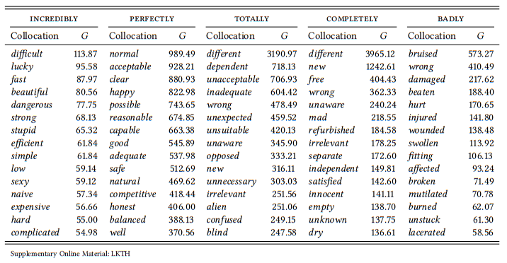
Kennedy finds, first, that there are some degree adverbs that do not appear to have restrictions concerning the adjectives they occur with (for example, very, really and particularly). However, most degree adverbs are clearly associated with semantically restricted sets of adjectives. The restrictions are of three broad types. First, there are connotational restrictions (some adverbs are associated primarily with positive words (e.g. perfectly) or negative words (e.g. utterly, totally; on connotation cf. also Section 7.2.3). Second, there are specific semantic restrictions (for example, incredibly, which is associated with subjective judgments), sometimes relating transparently to the meaning of the adverb (for example, badly, which is associated with words denoting damage or clearly, which is associated with words denoting sensory perception). Finally, there are morphological restrictions (some adverbs are used frequently with words derived by particular suffixes, for example, perfectly, which is frequently found with words derived by -able/-ible, or totally, whose collocates often contain the prefix un-). Table 7.10 illustrates these findings for 5 of the 24 degree adverbs and their top 15 collocates.
Unlike Kennedy, I have used the G statistic of the log-likelihood ratio test,6 and so the specific collocates differ from the ones he finds (generally, his lists include more low-frequency combinations, as expected given that he uses mutual information), but his observations concerning the semantic and morphological sets are generally confirmed.
This case study illustrates the exploratory design typical of collocational research as well as the kind of result that such studies yield and the observations possible on the basis of these results. By comparing the results reported here to Kennedy’s, you may also gain a better understanding as to how different association measures may lead to different results.
7.2.2 Lexical relations
One area of lexical semantics where collocation data is used quite intensively is the study of lexical relations – most notably, (near) synonymy (Taylor 2003, cf. below), but also polysemy (e.g. Yarowsky 1993, investigating the idea that associations exist not between words but between particular senses of words) and antonymy (Justeson & Katz 1991, see below).
7.2.2.1 Case study: Near synonyms
Natural languages typically contain pairs (or larger sets) of words with very similar meanings, such as big and large, begin and start or high and tall. In isolation, it is often difficult to tell what the difference in meaning is, especially since they are often interchangeable at least in some contexts. Obviously, the distribution of such pairs or sets with respect to other words in a corpus can provide insights into their similarities and differences.
Table 7.10: Selected degree adverbs and their collocates
One example of such a study is Taylor (2003), which investigates the synonym pair high and tall by identifying all instances of the two words in their subsense ‘large vertical extent’ in the LOB corpus and categorizing the words they modify into eleven semantic categories. These categories are based on semantic distinctions such as human vs. inanimate, buildings vs. other artifacts vs. natural entities, etc., which are expected a priori to play a role.
The study, while not strictly hypothesis-testing, is thus somewhat deductive. It involves two nominal variables; the independent variable TYPE OF ENTITY with eleven values shown in Table 7.11 and the dependent variable VERTICAL EXTENT ADJECTIVE with the values HIGH and TALL (assuming that people first choose something to talk about and then choose the appropriate adjective to describe it). Table 7.11 shows Taylor’s results (he reports absolute and relative frequencies, which I have used to calculate expected frequencies and χ2 components).
As we can see, there is little we can learn from this table, since the frequencies in the individual cells are simply too small to apply the χ2 test to the table as a whole. The only χ2 components that reach significance individually are those for the category HUMAN, which show that tall is preferred and high avoided with human referents. The sparsity of the data in the table is due to the fact that the analyzed sample is very small, and this problem is exacerbated by the fact that the little data available is spread across too many categories. The category labels are not well chosen either: they overlap substantially in several places (e.g., towers and walls are buildings, pieces of clothing are artifacts, etc.) and not all of them seem relevant to any expectation we might have about the words high and tall.
Taylor later cites earlier psycholinguistic research indicating that tall is used when the vertical dimension is prominent, is an acquired property and is a property of an individuated entity. It would thus have been better to categorize the corpus data according to these properties – in other words, a more strictly deductive approach would have been more promising given the small data set.
Alternatively, we can take a truly exploratory approach and look for differential collocates as described in Section 7.1.1 above – in this case, for differential noun collocates of the adjectives high and tall. This allows us to base our analysis on a much larger data set, as the nouns do not have to be categorized in advance.
Table 7.12 shows the top 15 differential collocates of the two words in the BNC.
Table 7.11: Objects described as tall or high in the LOB corpus (adapted from Taylor 2003)
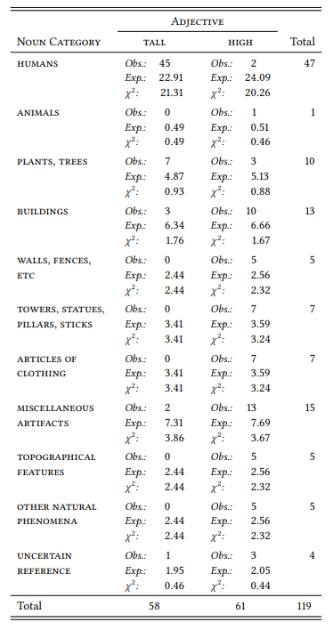
Table 7.12: Differential collocates for tall and high in the BNC
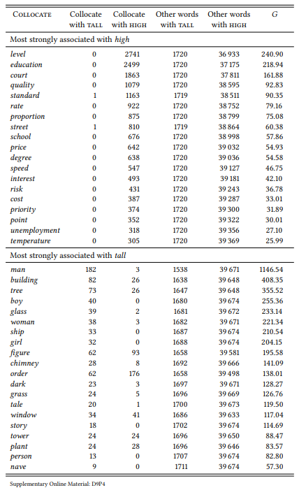
The results for tall clearly support Taylor’s ideas about the salience of the vertical dimension. The results for high show something Taylor could not have found, since he restricted his analysis to the subsense ‘vertical dimension’: when compared with tall, high is most strongly associated with quantities or positions in hierarchies and rankings. There are no spatial uses at all among its top differential collocates. This does not answer the question why we can use it spatially and in competition with tall, but it shows what general sense we would have to assume: one concerned not with the vertical extent as such, but with the magnitude of that extent (which, incidentally, Taylor notes in his conclusion).
This case study shows how the same question can be approached by a deductive or an inductive (exploratory) approach. The deductive approach can be more precise, but this depends on the appropriateness of the categories chosen a priori for annotating the data; it is also time consuming and therefore limited to relatively small data sets. In contrast, the inductive approach can be applied to a large data set because it requires no a priori annotation. It also does not require any choices concerning annotation categories; however, there may be a danger to project patterns into the data post hoc.
7.2.2.2 Case study: Antonymy
At first glance, we expect the relationship between antonyms to be a paradigmatic one, where only one or the other will occur in a given utterance. However, Charles & Miller (1989) suggest, based on the results of sorting tasks and on theoretical considerations, that, on the contrary, antonym pairs are frequently found in syntagmatic relationships, occurring together in the same clause or sentence. A number of corpus-linguistic studies have shown this to be the case (e.g. Justeson & Katz 1991, Justeson & Katz 1992, Fellbaum 1995; cf. also Gries & Otani 2010 for a study identifying antonym pairs based on their similarity in lexico-syntactic behavior).
There are differences in detail in these studies, but broadly speaking, they take a deductive approach: they choose a set of test words for which there is agreement as to what their antonyms are, search for these words in a corpus, and check whether their antonyms occur in the same sentence significantly more frequently than expected. The studies thus involve two nominal variables: SENTENCE (with the values CONTAINS TEST WORD and DOES NOT CONTAINS TEST WORD) and ANTONYM OF TEST WORD (with the values OCCUR IN SENTENCE and DOES NOT OCCUR IN SENTENCE). This seems like an unnecessarily complicated way of representing the kind of co-occurrence design used in the examples above, but I have chosen it to show that in this case sentences containing a particular word are used as the condition under which the occurrence of another word is investigated – a straightforward application of the general research design that defines quantitative corpus linguistics. Table 7.13 demonstrates the design using the adjectives good and bad (the numbers are, as always in this book, based on the tagged version of BROWN included with the ICAME collection and differ slightly from the ones reported in the studies discussed below).
Table 7.13: Sentential co-occurrence of good and bad in the BROWN corpus
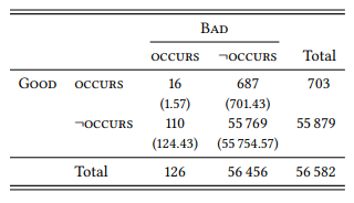
Good occurs significantly more frequently in sentences also containing bad than in sentences not containing bad, and vice versa (χ2 = 135.07, df = 1, p < 0.001). Justeson & Katz (1991) apply this procedure to 36 adjectives and get significant results for 25 of them (19 of which remain significant after a Bonferroni correction for multiple tests). They also report that in a larger corpus, the frequency of co-occurrence for all adjective pairs is significantly higher than expected (but do not give any figures). Fellbaum (1995) uses a very similar procedure with words from other word classes, with very similar results.
These studies only look at the co-occurrence of antonyms; they do not apply the same method to word pairs related by other lexical relations (synonymy, taxonomy, etc.). Thus, there is no way of telling whether co-occurrence within the same sentence is something that is typical specifically of antonyms, or whether it is something that characterizes word pairs in other lexical relations, too.
An obvious approach to testing this would be to repeat the study with other types of lexical relations. Alternatively, we can take an exploratory approach that does not start out from specific word pairs at all. Justeson & Katz (1991) investigate the specific grammatical contexts which antonyms tend to co-occur, identifying, among others, coordination of the type [ADJ and ADJ] or [ADJ or ADJ]. We can use such specific contexts to determine the role of co-occurrence for different types of lexical relations by simply extracting all word pairs occurring in the adjective slots of these patterns, calculating their association strength within this pattern as shown in Table 7.14 for the adjectives good and bad in the BNC, and then categorizing the most strongly associated collocates in terms of the lexical relationships between them.
Table 7.14: Co-occurrence of good and bad in the first and second slot of [ADJ1 and ADJ2 ]
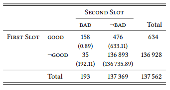
Note that this is a slightly different procedure from what we have seen before: instead of comparing the frequency of co-occurrence of two words with their individual occurrence in the rest of the corpus, we are comparing it to their individual occurrence in a given position of a given structure – in this case [ADJ and ADJ] (Stefanowitsch & Gries (2005) call this kind of design covarying collexeme analysis).
Table 7.15 shows the thirty most strongly associated adjective pairs coordinated with and in the BNC.
Clearly, antonymy is the dominant relation among these word pairs, which are mostly opposites (black/white, male/female, public/private, etc.), and sometimes relational antonyms (primary/secondary, economic/social, economic/political, social/political, lesbian/gay, etc.). The only cases of non-antonymic pairs are economic/monetary, which is more like a synonym than an antonym and the fixed expressions deaf /dumb and hon(ourable)/learned (as in honourable and learned gentleman/member/friend). The pattern does not just hold for the top 30 collocates but continues as we go down the list. There are additional cases of relational antonyms, like British/American and Czech/Slovak and additional examples of fixed expressions (alive and well, far and wide, true and fair, null and void, noble and learned), but most cases are clear antonyms (for example, syntactic/ semantic, spoken/written, mental/physical, right/left, rich/poor, young/old, good/ evil, etc.). The one systematic exceptions are cases like worse and worse (a special construction with comparatives indicating incremental change, cf. Stefanowitsch 2007b).
Table 7.15: Co-occurrence of adjectives in the first and second slot of [ADJ1 and ADJ2 ] (BNC)
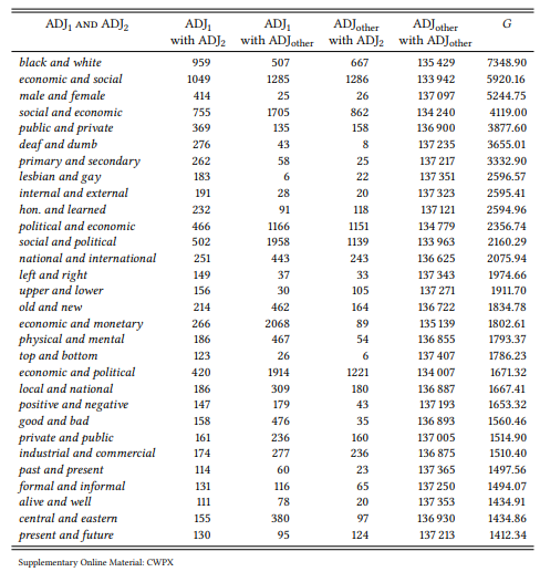
This case study shows how deductive and inductive domains may complement each other: while the deductive studies cited show that antonyms tend to co-occur syntagmatically, the inductive study presented here shows that words that co-occur syntagmatically (at least in certain syntactic contexts) tend to be antonyms. These two findings are not equivalent; the second finding shows that the first finding may indeed be typical for antonymy as opposed to other lexical relations.
The exploratory study was limited to a particular syntactic/semantic context, chosen because it seems semantically and pragmatically neutral enough to allow all kinds of lexical relations to occur in it. There are contexts which might be expected to be particularly suitable to particular kinds of lexical relations and which could be used, given a large enough corpus, to identify word pairs in such relations. For example, the pattern [ADJ rather than ADJ] seems semantically predisposed for identifying antonyms, and indeed, it yields pairs like implicit/explicit, worse/better, negative/positive, qualitative/quantitative, active/passive, real/apparent, local/national, political/economical, etc. Other patterns are semantically more complex, identifying pairs in more context-dependent oppositions; for example, [ADJ but not ADJ] identifies pairs like desirable/essential, necessary/sufficient, similar/identical, small/insignificant, useful/essential, difficult/impossible. The relation between the adjectives in these pairs is best described as pragmatic – the first one conventionally implies the second.
7.2.3 Semantic prosody
Sometimes, the collocates of a node word (or larger expressions) fall into a more or less clearly recognizable semantic class that is difficult to characterize in terms of denotational properties of the node word. Louw (1993: 157) refers to this phenomenon as “semantic prosody”, defined, somewhat impressionistically, as the “consistent aura of meaning with which a form is imbued by its collocates”.
This definition has been understood by collocation researchers in two different (but related) ways. Much of the subsequent research on semantic prosody is based on the understanding that this “aura” consists of connotational meaning (cf. e.g. Partington 1998: 68), so that words can have a “positive”, “neutral” or “negative” semantic prosody. However, Sinclair, who according to Louw invented the term,7 seems to have in mind “attitudinal or pragmatic” meanings that are much more specific than “positive”, “neutral” or “negative”. There are insightful terminological discussions concerning this issue (cf. e.g. Hunston 2007), but since the term is widely-used in (at least) these two different ways, and since “positive” and “negative” connotations are very general kinds of attitudinal meaning, it seems more realistic to accept a certain vagueness of the term. If necessary, we could differentiate between the general semantic prosody of a word (its “positive” or “negative” connotation as reflected in its collocates) and its specific semantic prosody (the word-specific attitudinal meaning reflected in its collocates).
7.2.3.1 Case study: True feelings
A typical example of Sinclair’s approach to semantic prosody, both methodologically and theoretically, is his short case study of the expression true feelings. Sinclair (1996b) presents a selection of concordance lines from the COBUILD corpus – Figure 7.1 shows a random sample from the BNC instead, as the COBUILD corpus is not accessible, but Sinclair’s findings are well replicated by this sample.
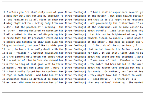
Figure 7.1: Concordance of true feelings (BNC, Sample)
On the basis of his concordance, Sinclair then makes a number of observations concerning the use of the phrase true feelings, quantifying them informally. He notes three things: first, the phrase is almost always part of a possessive (realized by pronoun, possessive noun phrase or of -construction). This is also true of the sample in Figure 7.1, with the exception of line 11 (where there is a possessive relation, but it is realized by the verb have).
Second, the expression collocates with verbs of expression (perhaps unsurprising for an expression relating to emotions); this, too, is true for our sample, where such verbs are found in 14 lines: reflect (line 2), show (lines 3, 9, 14, and 19), read (line 5), declare (line 6), disguise (line 7), reveal (line 8), hide (line 10), reveal (line 12), admit (line 13), give vent to (line 15), and tell (line 18).
Third, and most interesting, Sinclair finds that a majority of his examples express a reluctance to express emotions. In our sample, such cases are also noticeably frequent: I would argue that lines 2, 3, 5, 7, 8, 10, 12, 13, 14, 15, and 19 can be interpreted in this way, which would give us a slight majority of 11/20. (Your analysis may differ, as I have made my assessment rather intuitively, instead of coming up with an annotation scheme). In many cases, the reluctance or inability is communicated as part of the verb (like disguise, conceal and hide), in other cases it is communicated by negation of a verb of expression (like not admit in line 13) or by adjectives (like difficult to show in line 19).
Sinclair assumes that the denotational meaning of the phrase true feelings is “genuine emotions”. Based on his observations, he posits that, in addition, it has the semantic prosody “reluctance/inability to express emotions” – an attitudinal meaning much more specific than a general “positive” or “negative” connotation.
The methodological approach taken by Sinclair (and many others in his tradition) can yield interesting observations (at least, if applied very carefully): descriptively, there is little to criticize. However, under the definition of corpus linguistics adopted in this book, Sinclair’s observations would be just the first step towards a full analysis. First, note that Sinclair’s approach is quantitative only in a very informal sense – he rarely reports exact frequencies for a given semantic feature in his sample, relying instead on general statements about the frequency or rarity of particular phenomena. As we saw above, this is easy to remedy by simply determining the exact number of times that the phenomenon in question occurs in a given sample. However, such exact frequencies do not advance the analysis meaningfully: as long as we do not know how frequent a particular phenomenon is in the corpus as a whole, we cannot determine whether it is a characteristic property of the expression under investigation, or just an accidental one.
Specifically, as long as we do not know how frequent the semantic prosody ‘reluctance or inability to express’ is in general, we do not know whether it is particularly characteristic of the phrase true feelings. It may be characteristic, among other things, (a) of utterances concerning emotions in general, (b) of utterances containing the plural noun feelings, (c) of utterances containing the adjective true, etc.
In order to determine this, we have to compare our sample of the expression true feelings to related expressions that differ with respect to each property potentially responsible for the semantic prosody. For example, we might compare it to the noun feelings in order to investigate possibility (b). Figure 7.2 shows a sample of the expression [POSS feelings] (the possessive pronoun was included as it, too, may have an influence on the prosody and almost all examples of true feelings are preceded by a possessive pronoun).
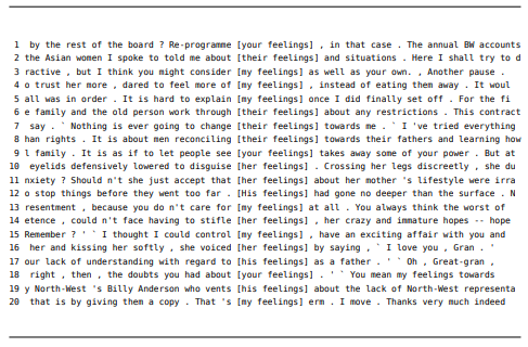
Figure 7.2: Concordance of [POSS feelings] (BNC, Sample)
The concordance shows that contexts concerning a reluctance or inability to express emotions are not untypical of the expression [POSS feelings] – it is found in four out of twenty lines in our sample, i.e. in 20 percent of all cases (lines 5, 10, 14, 15). However, it is nowhere near as frequent as with the expression true feelings. We can compare the two samples using the χ2 test. As Table 7.16 shows, the difference is, indeed, significant (χ2 = 5.23, df = 1, p < 0.05).
The semantic prosody is not characteristic of the noun feelings, even in possessive contexts. We can thus assume that it is not characteristic of utterances concerned with emotions generally. But is it characteristic of the specific expression true feelings, or would we find it in other contexts where a distinction between genuine and non-genuine emotions is made?
Table 7.16: Semantic prosody of true feelings and [POSS feelings]
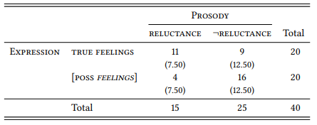
In order to answer this question, we have to compare the phrase to denotationally synonymous expressions, such as genuine emotions (which Sinclair uses to paraphrase the denotational meaning), genuine feelings, real emotions and real feelings. The only one of these expressions that occurs in the BNC more than a handful of times is real feelings. A sample concordance is shown in Figure 7.3.
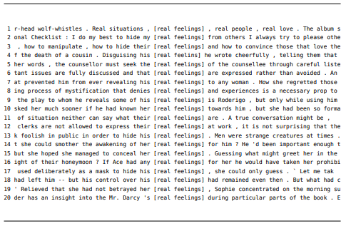
Figure 7.3: Concordance of real feelings (BNC, Sample)
Here, the semantic prosody in question is quite dominant – by my count, it is present in lines 2, 3, 4, 6, 7, 12, 13, 15, 17, 18 and 19, i.e., in 11 of 20 lines. This is the exact proportion also observed with true feelings, so even if you disagree with one or two of my categorization decisions, there is no significant difference between the two expressions.
It seems, then, that the semantic prosody Sinclair observes is not attached to the expression true feelings in particular, but that it is an epiphenomenon the fact that we typically distinguish between “genuine” (true, real, etc.) emotions and other emotions in a particular context, namely one where someone is reluctant on unable to express their genuine emotions. Of course, studies of additional expressions with adjectives meaning “genuine” modifying nouns meaning “emotion” might give us a more detailed and differentiated picture, as might studies of other nouns modified by adjectives like true (such as true nature, true beliefs, true intentions, etc.). Such studies are left as an exercise to the reader – this case study was mainly meant to demonstrate how informal analysis based on the inspection of concordances can be integrated into a more rigorous research design involving quantification and comparison to a set of control data.
7.2.3.2 Case study: The verb cause
A second way in which semantic prosody can be studied quantitatively is implicit in Kennedy’s study of collocates of degree adverbs discussed in Section 7.2.1 above. Recall that Kennedy discusses for each degree adverb whether a majority of its collocates has a positive or a negative connotation. This, of course, is a statement about the (broad) semantic prosody of the respective adverb, based not on an inspection and categorization of usage contexts, but on inductively discovered strongly associated collocates.
One of the earliest applications of this procedure is found in Stubbs (1995a). Stubbs studies, among other things, the noun and verb cause. He first presents the result of a manual extraction of all nouns (sometimes with adjectives qualifying them, as in the case of wholesale slaughter) that occur as subject or object of the verb cause or as a prepositional object of the noun cause in the LOB. He annotates them in their context of occurrence for their connotation, finding that approximately 80 percent are negative, 18 percent are neutral and 2 percent are positive. This procedure is still very close to Sinclairs approach of inspecting concordances, although is is stricter in terms of categorizing and quantifying the data.
Stubbs then notes that manual inspection and extraction becomes unfeasible as the number of corpus hits grows and suggests that, instead, we should first identify significant collocates of the word or expression we are interested in, and then categorize these significant collocates according to our criteria – note that this is the strategy we also used in Case Study 7.2.2.1 above in order to determine semantic differences between high and tall.
We will not follow Stubbs’ discussion in detail here – his focus is on methodological issues regarding the best way to identify collocates. Since we decided in Section 7.1.3 above to stick with the G statistic, this discussion is not central for us. Stubbs does not present the results of his procedure in detail and the corpus he uses is not accessible anyway, so let us use the BNC again and extract our own data.
Table 7.17 shows the result of an attempt to extract direct objects of the verb cause from the BNC. I searched for the lemma cause where it is tagged as a verb, followed by zero to three words that are not nouns (to take into account the occurrence of determiners, adjectives, etc.) and that are not the word by (in order to exclude passives like caused by negligence, fire, exposure, etc.), followed by a noun or sequence of nouns, not followed by to (in order to exclude causative constructions of the form caused the glass to break). This noun, or the last noun in this sequence, is assumed to be the direct object of cause. The twenty most frequent nouns are shown in Table 7.17, Column (a).
These collocates clearly corroborate Stubbs’ observation about the negative semantic prosody of cause. We could now calculate the association strength between the verb and each of these nouns to get a better idea of which of them are significant collocates and which just happen to be frequent in the corpus overall. It should be obvious, however, that the nouns in Table 7.17, Column (a) are not generally frequent in the English language, so we can assume here that they are, for the most part, significant collocates.
But even so, what does this tell us about the semantic prosody of the verb cause? It has variously been pointed out (for example, by Louw & Chateau 2010) that other verbs of causation also tend to have a negative semantic prosody – the direct object nouns of bring about in Table 7.17, Column (b) and lead to in Table 7.17, Column (c) corroborate this. The real question is, again, whether it is the specific expression [cause NP] that has the semantic prosody in question, or whether this prosody is found in an entire semantic domain – perhaps speakers of English have a generally negative view of causation.
In order to determine this, it might be useful to compare different expressions of causation to each other rather than to the corpus as a whole – to perform a differentiating collocate analysis: just by inspecting the frequencies in Table 7.17, it seems that the negative prosody is much weaker for bring about and lead to than for cause, so, individually or taken together, they could serve as a baseline against which to compare cause.
Table 7.17: Noun collocates of three expressions of causation
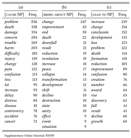
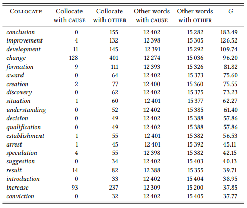
Table 7.18 shows the results of a differential collocate analysis between cause on the one hand and the combined collocates of bring about and lead to on the other.
Table 7.18: Differential collocates for cause compared to bring about/lead to in the BNC
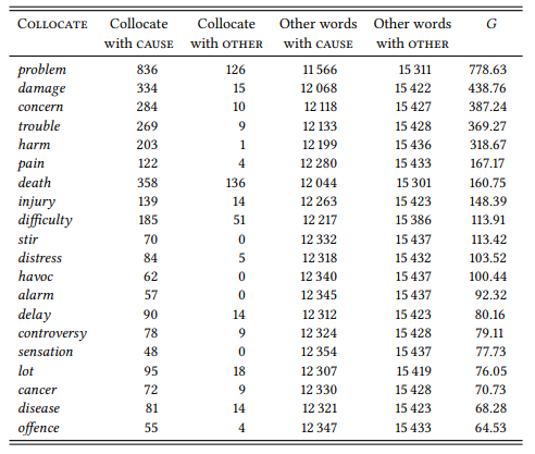
The negative prosody of the verb cause is even more pronounced than in the frequency list in Table 7.17: Even the two neutral words change and increase have disappeared. In contrast, the combined differential collocates of bring about and lead to as compared to cause, shown in Table 7.19 are neutral or even positive.
We can thus conclude, first, that all three verbal expressions of causation are likely to be used to some extent with direct object nouns with a negative connotation. However, it is only the verb cause that has a negative semantic prosody. Even the raw frequencies of nouns occurring in the object position of the three expressions suggest this: while cause occurs almost exclusively with negatively connoted nouns, bring about and lead to are much more varied. The differential collocate analysis then confirms that within the domain of causation, the verb cause specializes in encoding negative caused events, while the other two expressions encode neutral or positive events. Previous research (Louw & Chateau 2010) misses this difference as it is based exclusively on the qualitative inspection of concordances.
Table 7.19: Differential collocates for bring about/lead to compared to cause in the BNC
Thus, the case study shows, once again, the need for strict quantification and for research designs comparing the occurrence of a linguistic feature under different conditions. There is one caveat of the procedure presented here, however: while it is a very effective strategy to identify collocates first and categorize them according to their connotation afterwards, this categorization is then limited to an assessment of the lexically encoded meaning of the collocates. For example, problem and damage will be categorized as negative, but a problem does not have to be negative – it can be interesting if it is the right problem and you are in the right mood (e.g. [O]ne of these excercises caused an interesting problem for several members of the class [Aiden Thompson, Who’s afraid of the Old Testament God?]). Even damage can be a good thing in particular contexts from particular perspectives (e.g. [A] high yield of intact PTX [...] caused damage to cancer cells in addition to the immediate effects of PDT [10.1021/acs.jmedchem.5b01971]). Even more likely, neutral words like change will have positive or negative connotations in particular contexts, which are lost in the proces of identifying collocates quantitatively.
Keeping this caveat in mind, however, the method presented in this case study can be applied fruitfully in more complex designs than the one presented here. For example, we have treated the direct object position as a simple category here, but Stefanowitsch & Gries (2003) present data for nominal collocates of the verb cause in the object position of different subcategorization patterns. While their results corroborate the negative connotation of cause also found by Stubbs (1995a), their results add an interesting dimension: while objects of cause in the transitive construction (cause a problem) and the prepositional dative (cause a problem to someone) refer to negatively perceived external and objective states, the objects of cause in the ditransitive refer to negatively experienced internal and/or subjective states. Studies on semantic prosody can also take into account dimensions beyond the immediate structural context – for example, Louw & Chateau (2010) observe that the semantic prosody of cause is to some extent specific to particular language varieties, and present interesting data suggesting that in scientific writing it is generally used with a neutral connotation.
7.2.4 Cultural analysis
In collocation research, a word (or other element of linguistic structure) typically stands for itself – the aim of the researcher is to uncover the linguistic properties of a word (or set of words). However, texts are not just manifestations of a language system, but also of the cultural conditions under which they were produced. This allows corpus linguistic methods to be used in uncovering at least some properties of that culture. Specifically, we can take lexical items to represent culturally defined concepts and investigate their distribution in linguistic corpora in order to uncover these cultural definitions. Of cou rse, this adds complexity to the question of operationalization: we must ensure that the words we choose are indeed valid representatives of the cultural concept in question.
7.2.4.1 Case study: Small boys, little girls
Obviously, lexical items used conventionally to refer to some culturally relevant group of people are plausible representatives of the cultural concept of that group. For example, some very general lexical items referring to people (or higher animals) exist in male and female versions – man/woman, boy/girl, lad/lass, husband/wife, father/mother, king/queen, etc. If such word pairs differ in their collocates, this could tell us something about the cultural concepts behind them. For example, Stubbs (1995b) cites a finding by Baker & Freebody (1989), that in children’s literature, the word girl collocates with little much more strongly than the word boy, and vice versa for small. Stubbs shows that this is also true for balanced corpora (see Table 7.20; again, since Stubbs’ corpora are not available, I show frequencies from the BNC instead but the proportions are within a few percent points of his). The difference in associations is highly significant (χ2 = 217.66, df = 1, p < 0.001).
Table 7.20: Small and little girls and boys (BNC)
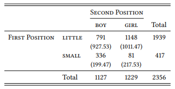
This part of Stubbs’ study is clearly deductive: He starts with a hypothesis taken from the literature and tests it against a larger, more representative corpus. The variables involved are, as is typical for collocation studies, nominal variables whose values are words.
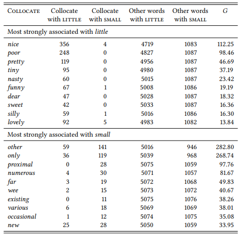
Stubbs argues that this difference is due to different connotations of small and little which he investigates on the basis of the noun collocates to their right and the adjectival and adverbial collocates to the left. Again, instead of Stubbs’ original data (which he identifies on the basis of raw frequency of occurrence and only cites selectively), I use data from the BNC and the G test statistic. Table 7.21 shows the ten most strongly associated noun collocates to the right of the node word and Table 7.22 shows the ten most strongly associated adjectival collocates to the left.
Table 7.21: Nominal collocates of little and small at R1 (BNC)
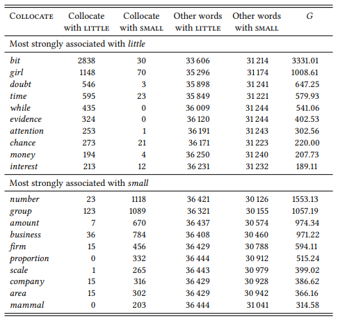
Table 7.22: Adjectival collocates of little and small at L1 (BNC)
This part of the study is more inductive. Stubbs may have expectations about what he will find, but he essentially identifies collocates exploratively and then interprets the findings. The nominal collocates show, according to Stubbs, that small tends to mean ‘small in physical size’ or ‘low in quantity’, while little is more clearly restricted to quantities, including informal quantifying phrases like little bit. This is generally true for the BNC data, too (note, however, the one exception among the top ten collocates – girl).
The connotational difference between the two adjectives becomes clear when we look at the adjectives they combine with. The word little has strong associations to evaluative adjectives that may be positive or negative, and that are often patronizing. Small, in contrast, does not collocate with evaluative adjectives.
Stubbs sums up his analysis by pointing out that small is a neutral word for describing size, while little is sometimes used neutrally, but is more often “nonliteral and convey[s] connotative and attitudinal meanings, which are often patronizing, critical, or both.” (Stubbs 1995b: 386). The differences in distribution relative to the words boy and girl are evidence for him that “[c]ulture is encoded not just in words which are obviously ideologically loaded, but also in combinations of very common words” (Stubbs 1995b: 387).
Stubbs remains unspecific as to what that ideology is – presumably, one that treats boys as neutral human beings and girls as targets for patronizing evaluation. In order to be more specific, it would be necessary to turn around the perspective and study all adjectival collocates of boy and girl. Stubbs does not do this, but Caldas-Coulthard & Moon (2010) look at adjectives collocating with man, woman, boy and girl in broadsheet and yellow-press newspapers. In order to keep the results comparable with those reported above, let us stick with the BNC instead. Table 7.23 shows the top ten adjectival collocates of boy and girl.
The results are broadly similar in kind to those in Caldas-Coulthard & Moon (2010): boy collocates mainly with neutral descriptive terms (small, lost, big, new), or with terms with which it forms a fixed expression (old, dear, toy, whipping). There are the evaluative adjectives rude (which in Caldas-Coulthard and Moon’s data is often applied to young men of Jamaican descent) and its positively connoted equivalent naughty. The collocates of girl are overwhelmingly evaluative, related to physical appearance. There are just two neutral adjective (other and dead, the latter tying in with a general observation that women are more often spoken of as victims of crimes and other activities than men). Finally, there is one adjective signaling marital status. These results also generally reflect Caldas-Coulthard and Moon’s findings (in the yellow-press, the evaluations are often heavily sexualized in addition).
Table 7.23: Adjectival collocates of boy and girl at L1 (BNC)
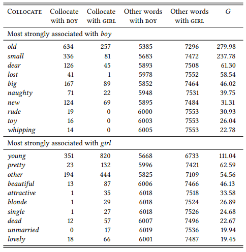
This case study shows how collocation research may uncover facts that go well beyond lexical semantics or semantic prosody. In this case, the collocates of boy and girl have uncovered a general attitude that sees the latter as up for constant evaluation while the former are mainly seen as a neutral default. That the adjectives dead and unmarried are among the top ten collocates in a representative, relatively balanced corpus, hints at something darker – a patriarchal world view that sees girls as victims and sexual partners and not much else (other studies investigating gender stereotypes on the basis of collocates of man and woman are Gesuato (2003) and Pearce (2008)).
7 Louw attributes the term to John Sinclair, but Louw (1993) is the earliest appearance of the term in writing. However, Sinclair is clearly the first to discuss the phenomenon itself systematically, without giving it a label (e.g. Sinclair 1991: 74–75).


