2.9: Exercise- Averaged ERPs

We’re now finally ready to create the averaged ERPs for this participant. First make sure that the dataset from the previous exercise is loaded (6_N400_preprocessed_filt_elist_bins_be_ar). Then select EEGLAB > ERPLAB > Compute averaged ERPs. A window will pop up that allows you to specify a variety of options for the averaging process, which is shown in Screenshot 2.15.

Averaging Options

The first and most essential value is an index for the dataset that contains the epoched EEG to be averaged. You can see the list of datasets that are currently loaded into EEGLAB in the Datasets menu (see the upper left portion of Screenshot 2.15). The currently active dataset is indicated with a check mark (and is ordinarily the most recently loaded or created dataset), and by default this is the dataset that will be used for averaging.

Screenshot 2.15

The datasets that are loaded depend on what you’ve done since launching EEGLAB. And your Datasets menu will look different from mine, because mine has a bunch of datasets that were created as I was trying out different things while creating the exercises in this chapter. We want to average the epoched dataset in which the epochs with artifacts have been marked (6_N400_preprocessed_filt_elist_bins_be_ar). For me, this is Dataset 6 in the Datasets menu, but it is probably a different dataset in your Datasets menu. In the GUI for the averaging routine, make sure that the right dataset number is listed in the text field at the top (EEG Dataset(s) Index).

Dealing with multiple datasets for a given participant

Imagine that you are running an EEG recording session and a fire alarm starts ringing halfway through the session. You would need to stop recording, disconnect the participant, and head to safety. But after 5 minutes, the alarm stops and you’re allowed back into the lab. You reconnect the participant and resume the recording, but with the data in a new file. How do you average together the trials from the two files?

Another possibility is that you run an experiment with 10 different trial blocks, and you create a different EEG recording file for each block. Again, you need to be able to average the data across multiple blocks.

One way to accomplish this is to combine the datasets into a single dataset with EEGLAB > Edit > Append datasets. But if you want to keep the datasets separate (e.g., so you don’t overload your computer’s memory with huge datasets), you can actually specify more than one dataset in the text box at the top of the averaging GUI. The datasets that you specify will be treated like a single large dataset during the averaging process.

The next section of the averaging GUI controls how artifacts are treated during the averaging process. The default option, which you should make sure is selected, is Exclude epochs marked during artifact detection. We also provide options for including all of the epochs (whether or not they are marked for artifacts) or for including only the marked epochs; these options are used only rarely.

You should also make sure that there is a check mark in the box labeled Exclude epochs that contain either “boundary” or invalid events. A boundary is a special event code that indicates a discontinuity in the EEG. For example, imagine that the data collection was temporarily paused 300 ms after the onset of an event because the participant asked for a short break, and then it was restarted again a minute later. A boundary code would be inserted into the data at the time of the pause. We wouldn't want to include that trial, and so we exclude trials with boundary events. Another possibility is that the enable flag in the EventList was set to zero for the time-locking event (e.g., because you realized that the participant had fallen asleep during the last part of the experiment and you therefore disabled the events during that period after the session was over). These trials should also be excluded.

ERPLAB can calculate some measures of data quality during the averaging process, and the Data Quality section of the averaging GUI allows you to control this process. Just leave it set to On – default parameters. ERPLAB can also compute power spectra during the averaging process, but you should leave the Power Spectra options off for the present exercise.

Creating and Saving an ERPset

Once you have everything set properly in the averaging GUI, you can click RUN to create the averaged ERPs. You’ll then see a window that allows you to save the averaged ERPs, which are stored in an ERPset (as illustrated earlier in Figure 2.2). You should name the ERPset 6_ERP (because this is the ERP data from Participant 6). That’s the name that will show up in the ERPsets menu. You can also save the ERPset on your hard drive as a file. To do this, activate the Save ERP as button. The name of the ERPset in memory does not need to be the same as the name of the file, but it’s usually a good idea to use the same name for both. You can accomplish this by clicking the same as erpname button, which will put 6_ERP into the text box for the filename. Once you have everything set, you can click the OK button. If you look in the ERPsets menu in the main EEGLAB GUI, you’ll see that the new ERPset is now listed as ERPset 1: 6_ERP.

If you look in the Matlab command window, you’ll see that the averaging routine printed a bunch of information when it finished. Here’s the last part of what it printed:

TOTAL:
The dataset 6_N400_preprocessed_filt_elist_bins_be_ar has a 38.5 % of discarded trialsSummary per bin:
Bin 1 was created with a 41.7 % of rejected trials
Bin 1 was created with a 0.0 % of invalid trials
Bin 2 was created with a 55.0 % of rejected trials
Bin 2 was created with a 0.0 % of invalid trials
Bin 3 was created with a 29.6 % of rejected trials
Bin 3 was created with a 0.0 % of invalid trials
Bin 4 was created with a 26.3 % of rejected trials
Bin 4 was created with a 0.0 % of invalid trials
---------------------------------------------------
Data Quality measure of aSME
Median value of 1.0008 at elec FP2, and time-window 0:100ms, on bin 1, Prime word, related to subsequent target word
Min value of 0.16593 at elec Oz, and time-window -200:100ms, on bin 1, Prime word, related to subsequent target word
Max value of 3.5935 at elec F4, and time-window 600:700ms, on bin 3, Target word, related to previous prime, followed by correct response

You should always look at this information in the command window. First, it allows you to verify that the expected number of trials were rejected because of artifacts. Second, it allows you to see if there were any invalid trials (e.g., trials on which the enable flag in the EventList was set so zero). Third, it provides a summary of some data quality metrics (which will be described in a later section).

Viewing the Averaged ERP Waveforms

Now let’s plot the averaged ERP waveforms. Select EEGLAB > ERPLAB > Plot ERP > Plot ERP waveforms, and a big complicated window will pop up with lots of options for controlling the plotting. Click the RESET button near the bottom to reset it to the default parameters. To keep things simple, we’ll start by looking at the ERPs to the prime words, which are stored in Bin 3 (for targets that were related to the preceding prime) and Bin 4 (for targets that were unrelated to the preceding prime). To specify that we want to plot just Bins 3 and 4, uncheck the button in the top left of the GUI labeled all bins and type 3 4 into the text box underneath (as in Screenshot 2.16). You could instead click the Browse button to see a list of the bins.

Screenshot 2.16

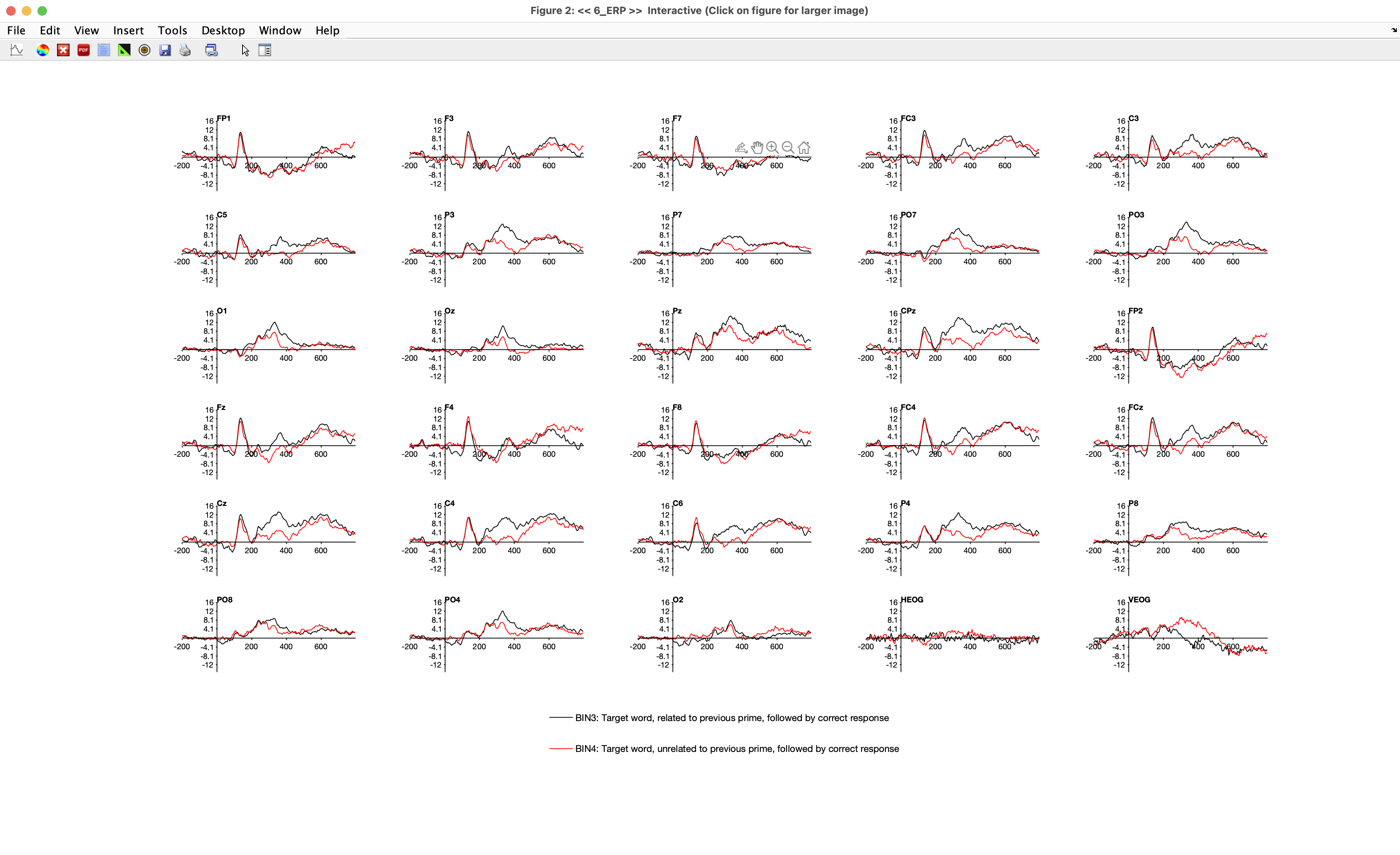
Now click PLOT to see the waveforms. It should look something like Screenshot 2.17. If you’re not used to looking at ERP waveforms, the plot may look like a chimpanzee threw a plate of spaghetti on the wall, but once you gain some expertise it will be easy for you to comprehend what you’re seeing. I always recommend starting by looking at the prestimulus baseline period. Note that it’s relatively flat compared to the poststimulus period. In theory, the prestimulus period should contain only random noise in the single-trial EEG epochs, and if we average together enough epochs, the noise will “average out” to zero. It never actually reaches a perfectly flat line with a finite number of trials. (This would be a good time to remind yourself of how many trials were in each bin.) Also, there may be a tilt in the waveform during the prestimulus period as a result of overlapping ERP activity from the previous stimulus or anticipatory activity.

Screenshot 2.17

In this particular example, the prestimulus baseline period looks quite good. The residual noise after averaging is relatively small compared to the ERPs in the poststimulus period, and there is no obvious tilt. I wish they always looked this good. I chose Participant 6 for this chapter because the data were very nice. In later exercises, you’ll see participants with much noisier data.

Now take a look at the poststimulus period. Start by looking at the CPz channel, which is the channel where the N400 is typically largest and is the channel shown in the grand average in Figure 2.1. (If you want a zoomed-in view, you can single-click the channel label to get a new window that shows only this channel.) You can see that there is a large broad positive voltage for the targets that were related to the preceding prime word, extending from approximately 200 ms until the end of the epoch at 800 ms. For the targets that were unrelated to the preceding prime, the voltage is more negative (less positive) during much of this period. The existing evidence indicates that both the related and unrelated target words produce essentially the same activity, including the broad positive voltage, but that the unrelated words also produce an additional negative voltage (the N400) that is added onto the broad positive voltage. So, even though the voltage remains above zero for the unrelated targets, the difference between the related and unrelated targets appears to be largely the result of the addition of an N400 component for the unrelated targets. This N400 activity appears to reflect the additional work the brain must do to process a word that is not related to the concepts that were already active when the word was presented (for a review of the N400 and other language-related ERP components, see Swaab et al., 2012).

Now take a look at the other channels. You’ll see that waveforms in channels near CPz (e.g., Cz, C3, C4, Pz, P3, C4, P4) look quite similar to the CPz waveforms, but the waveforms in more distant channels (e.g., Fp1, Fp2, Oz) look quite different. This is because the resistance of the skull is high (especially relative to the underlying cortex and overlying scalp), which causes the voltages to spread widely before they reach the electrodes.

If this is the first time you’ve ever created averaged ERPs, I hope you have a real sense of accomplishment and awe. You are looking at voltages created by neurons in the brain of a living human being who looked at pairs of words and decided whether the second word in each pair (the target) was related or unrelated to the first word (the prime). A tremendous amount of brain power and knowledge was needed for this participant to take the light emitted by the pixels on the computer screen, organize this light into letters and words, recognize the words, access their meanings, and compare them. And you are looking at the actual voltages created by the neurons as the brain carried out these processes. That is, the ERPs are the extracellular voltages produced by cortical pyramidal neurons as a result of neurotransmission, which (amazingly!) are able to pass through the brain, meninges, skull, and scalp to our recording electrodes. I’ve been recording and analyzing ERPs for almost 40 years, and this still gives me chills!!!

Viewing the Prime Words

Now let’s look at the averaged ERP waveforms for the prime words. Select EEGLAB > ERPLAB > Plot ERP > Plot ERP waveforms, and set it up just as you did to look at the target words except specify 1 2 in the Bins to plot section. Bin 1 is the ERP for prime words that are followed by a related target word, and Bin 2 is the ERP for prime words that are followed by an unrelated target word. Unless the participant had ESP, these ERPs should be equivalent except for random noise. How could the brain response to a given word vary according to the nature of a word that presented later in time?

Click the PLOT button to see the waveforms for Bins 1 and 2. If you look at the CPz channel, where the N400 effect was largest for the target words, you’ll see that the waveforms for the two prime bins are pretty similar until about 400 ms poststimulus (see Screenshot 2.18). Then, the waveform becomes slightly more negative for primes followed by related words than for primes followed by unrelated words. Logically, this small difference must just be random noise in the data.

Screenshot 2.18

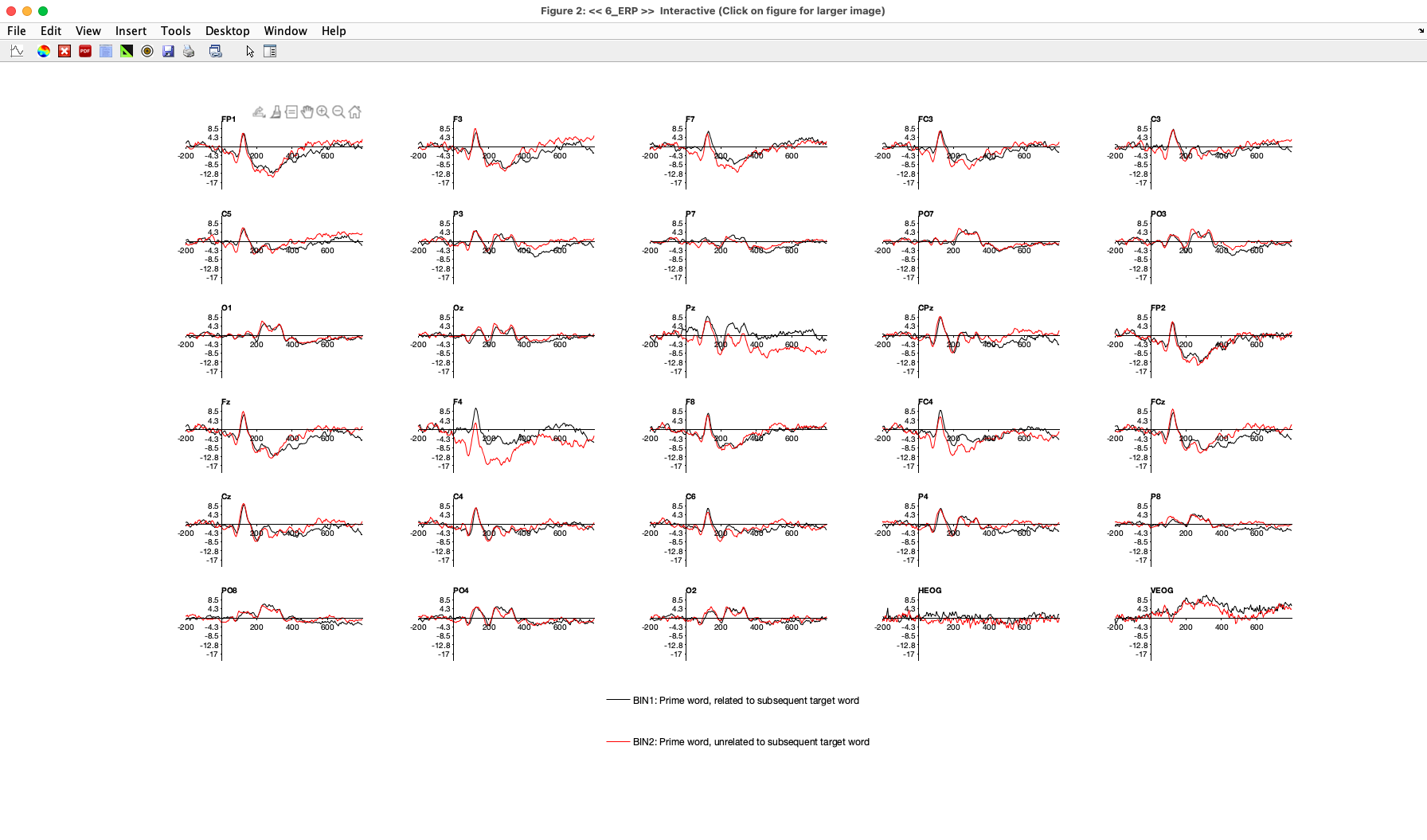
Now look at the F4 channel. You should see a large difference between Bins 1 and 2, beginning right around the onset of the prime word (0 ms). This absolutely must be noise, because it takes at least 50 ms for visual information to reach the cortex and generate an ERP. A similar but somewhat smaller early effect can be seen at the Pz electrode site.

Noise is an inevitable fact of life in ERP studies. After all, we’re trying to measure voltages produced by tiny neurons in the cerebral cortex with electrodes placed on the skin, and there is a big thick skull between the neurons and the skin. Also, the brain signals are only a few millionths of a volt once they reach the scalp, where they’re mixed with other signals such as skin potentials, muscle activity, and induced voltages from computers and other electrical devices in the recording environment. When you read journal articles, you don’t usually get to see the single-participant data. Instead, you see grand averages, which have much less noise. Even without noise, the ERP waveforms from different people often look quite different from each other (probably due to individual differences in how the cortex is folded up in the brain). So, don’t be surprised when the single-participant data you see in this book or in your own studies look quite different from the grand average waveforms in published papers.