The eyeblink artifacts you saw in the previous exercise are huge relative to the EEG, and these artifacts can be a real problem. They can make it difficult to see the actual brain activity, and we need a way to deal with them. In the published version of the ERP CORE experiments, we used a method called Independent Component Analysis (ICA) to estimate and remove the artifactual voltages, leaving behind the uncontaminated EEG. ICA is both slow and complicated, so we won’t use it in this chapter (but we’ll cover it in detail in Chapter 9). Instead, we’ll use a cruder approach called artifact rejection. In this approach, we use a simple algorithm to identify which epochs are contaminated by eyeblinks. We’ll then mark these epochs by setting a flag in the EventList. Later, when we make the averaged ERPs, we’ll simply leave out the epochs in which this flag has been set.
There is a lot to know about artifacts and artifact rejection, and this topic will be covered in detail in Chapter 8. For now, we’ll take a very simple approach in which we’ll check every epoch to see if the voltage exceeds ±100 µV in any channel. If the voltage exceeds this range in a given epoch, we’ll flag that epoch for rejection. We call this stage of the process artifact detection rather than artifact rejection, because we’re simply marking the epochs with artifacts so that they will be excluded when we get to the averaging step.
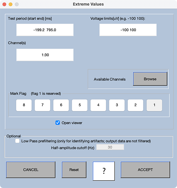
For this exercise, make sure that the dataset created during the previous exercise (6_N400_preprocessed_filt_elist_bins_be) is loaded in EEGLAB. Then select EEGLAB > ERPLAB > Artifact detection in epoched data > Simple voltage threshold. In the window that pops up, enter -100 100 as the voltage limits, make sure that only the Flag 1 button is selected (slightly darker gray), and make sure that the other parameters match those shown in Screenshot 2.13).
Screenshot 2.13
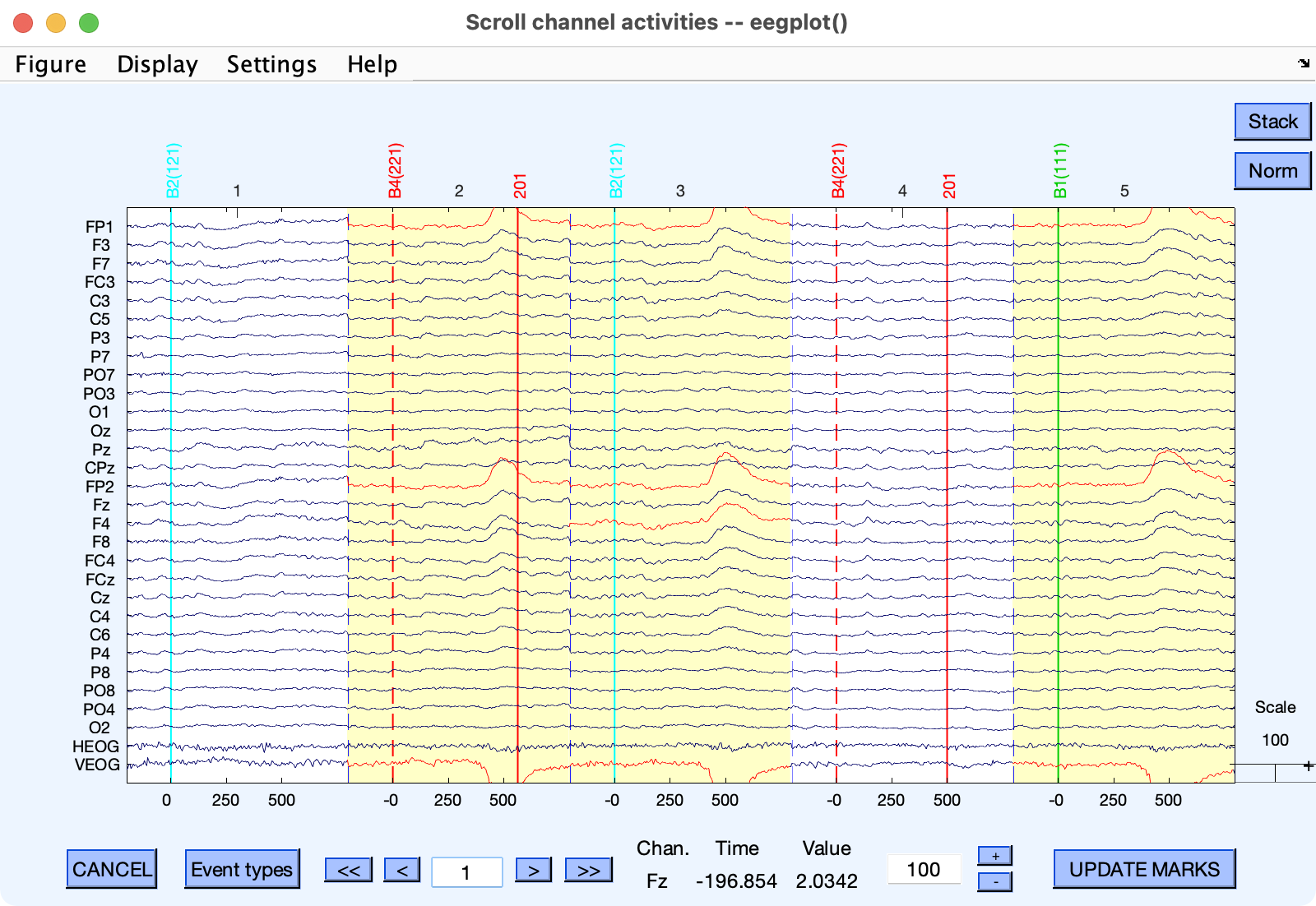
When you click the ACCEPT button, ERPLAB will test every epoch for artifacts, and then two windows will pop up. One is the usual window asking what you would like to do with the new dataset. The other is the usual EEG plotting window, but now any epoch with an artifact is highlighted with a yellow background (see Screenshot 2.14). The idea is that you’ll first use the EEG plotting window to make sure that ERPLAB did an adequate job of detecting artifacts. Then, if everything looks fine, you’ll click OK in the “save” window to keep the new dataset. Often, however, your visual inspection of the EEG will indicate that some adjustments need to be made to the artifact detection parameters. For example, you might see that some blinks were missed because they were too small. You might then reduce the voltage limits (e.g., setting them to ±90 instead of ±100 in the window shown in Screenshot 2.13) and run the artifact detection procedure again. Chapter 8 describes this process in detail.
Screenshot 2.14
Verifying that the Epochs with Artifacts Have Been Flagged
Go ahead and take a look at the EEG in the plotting window, using a vertical scale of 100 µV as shown in Screenshot 2.14. In the first screen of data, you can see that the second, third, and fifth epochs are marked as containing artifacts. The individual channels that exceeded our ±100 µV limits are drawn in red, and the epochs containing an artifact in one or more channels have a yellow background. We will exclude an entire epoch from our averages even if it contains an artifact in only one channel. The reason is that the artifact may not be easily visible in all channels in the raw EEG, but it might still be large enough to distort our data. Also, it would be a little weird if our averaged ERPs were based on different trials for different channels.
Now scroll through all of the data in the EEG plotting window and check to see if there are any epochs 1) that contain large artifacts that are not marked for rejection or 2) that do not contain large artifacts and are nonetheless marked for rejection.
When I go through the data, it looks pretty good, but I did find a few epochs that contain smallish eyeblink artifacts but were not marked for rejection (e.g., epochs 9, 154, and 201). They all contain voltage deflections in the VEOG channel that have the same basic shape as the eyeblinks that were flagged for rejection, along with an opposite-polarity deflect in the Fp1 and Fp2 electrodes. As will be discussed in Chapter 8, this pattern is characteristic of eyeblinks. So, the very simple approach that we’ve used to detect eyeblinks in this exercise is pretty good but not perfect. We’ll talk about better approaches in Chapter 8.
This participant blinked a lot, more than is typical, so a lot of trials will be excluded from our averaged ERPs. This will in turn reduce the signal-to-noise ratio of the averaged ERPs, making it more difficult to precisely quantify the N400 amplitude. To see exactly how many trials were marked for rejection, go to the main Matlab GUI and look in the command window. You’ll see that the artifact detection routine produced a table showing the number and percentage of accepted and rejected trials for each bin, as well as the total across bins. (Don’t worry about the columns labeled F2, F3, etc., which will be discussed in Chapter 8). You’ll see that 38.5% of trials were rejected across bins. Ordinarily, my lab “throws out” any participant for whom more than 25% of trials were rejected (see Chapter 6 in Luck, 2014). However, this experiment was designed to be analyzed using artifact correction instead of artifact rejection (see Chapter 9), so we didn’t actually need to exclude this participant. By the way, you can print this table of values at a later time if you’d like by selecting EEGLAB > ERPLAB > Summarize artifact detection.
Now that you’ve looked through the epochs and the number of trials with artifacts, you can go to the window that asks What do you want to do with the new dataset? and click OK to save this dataset as 6_N400_preprocessed_filt_elist_bins_be_ar. Save the dataset to your hard drive if you’re not going to do the next exercise right away.