The next step in processing Subject 6’s data is quite simple, and it involves two operations that are done together in a single step. One of these operations is extracting a fixed-length epoch for each event that has been assigned to a bin. If you’re not quite sure what this means, see Figure A1.3 in Appendix 1). As shown in Figure 2.1, we will be looking at the data from 200 ms prior to stimulus onset through 800 ms after stimulus onset. Consequently, for each trial we need to extract an epoch that starts 200 ms before the time-locking event code and extends until 800 ms after the event code.
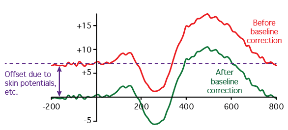
The second operation will be baseline correction, which is a way of dealing with the DC voltage offsets. As shown in Figure 2.3, we use the average voltage during the prestimulus period as an estimate of the offset, and we shift the whole waveform upward or downward by this amount. Ordinarily, this is done on epoched EEG data, but ERPLAB also allows you to perform correction on averaged ERP waveforms as well.
Figure 2.3. Baseline correction procedure. The mean voltage during the prestimulus period (from -200 to 0 ms in this example) is used as an estimate of the voltage offset. This value is simply subtracted from each point in the waveform to create the corrected waveform.
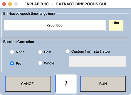
To perform these steps on our example data, make sure that the dataset created during the previous exercise (6_N400_preprocessed_filt_elist_bins) is loaded in EEGLAB. Then select EEGLAB > ERPLAB > Extract bin-based epochs. In the window that pops up, enter -200 800 as the time range and select Pre for baseline correction (as in Screenshot 2.12). The time window values tell the routine that you want the epochs to start 200 ms before stimulus onset and extend for 800 ms after stimulus onset, for a total epoch length of 1000 ms. The baseline correction parameter tells the routine that you want to use the entire prestimulus interval (-200 to 0 ms) as the baseline period. Once you’ve set these parameters, click RUN. As usual, accept the default settings when asked What do you want to do with the new dataset? The new dataset should be named 6_N400_preprocessed_filt_elist_bins_be. Save it to your hard drive if you’re not going to do the next exercise right away.
Screenshot 2.12
Looking at the Epoched Dataset
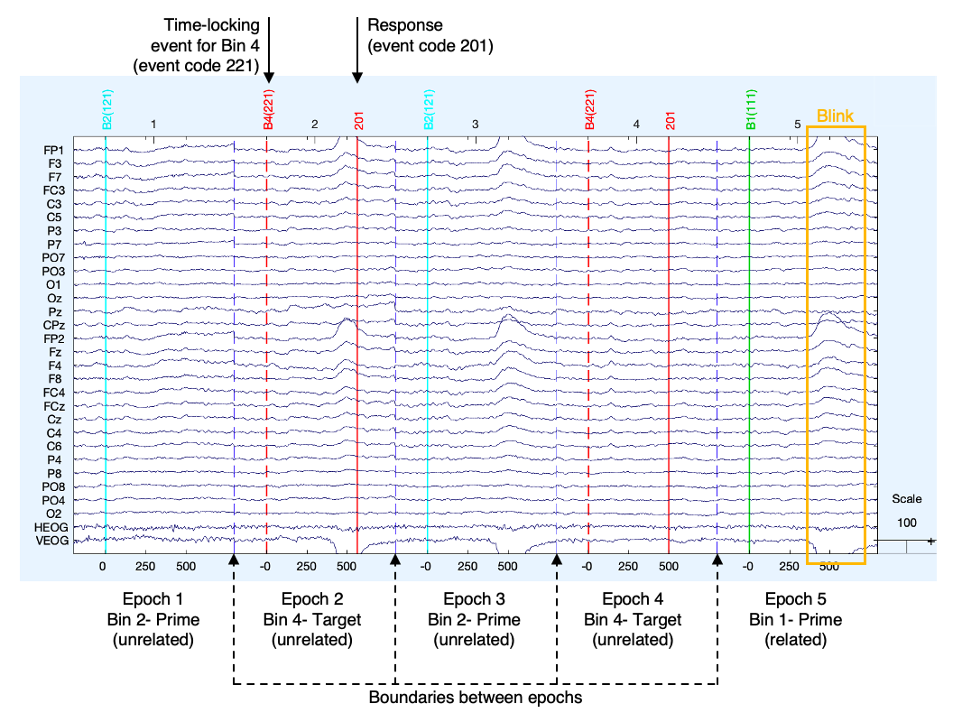
Now let’s see what happened when you ran this routine by selecting EEGLAB > Plot > Channel data (scroll). You should set the vertical scale to 100 in the plotting window, but you don’t need to remove the DC offset (because it was removed by the baseline correction procedure). The result should look like the plot in Figure 2.4. By default, the EEG plotting window shows 5 individual epochs, but it looks a lot like one continuous EEG waveform for each channel until you look closely. There is a dashed vertical line between each epochs, 200 ms before the event codes that were used for time locking (because we specified a 200-ms prestimulus period when we epoched the data).
Figure 2.4. Plot of epoched EEG data. It looks like continuous data, but the dashed horizontal lines indicate boundaries between epochs.
For example, look at the event code labeled B4(221), which corresponds to item #4 in the EventList (line 34) shown in Screenshot.2.10. This event code corresponds to a target word, and it was assigned to Bin 4 when you ran BINLISTER. The event code label now contains both the bin number (B4) and the original event code (221). If you look at the labels on the X axis, you’ll see that this event is at time zero, because it’s the time-locking event for this epoch. When we create our averaged ERPs, all the epochs labeled B1 will be averaged together to form Bin 1 (whether the actual event code was 111 or 112), all the epochs labeled B2 will be averaged together to form Bin 2 (whether the actual event code was 121 or 122), etc.
The next event code is labeled 201. This was the response to the target word. We’re not using it as the time-locking point for any bins, so it does not have a bin number. However, the information about the event is still present, so you can see the event code in the EEG plotting window.
Scroll through the epochs using the >> button at the bottom of the plotting window. Notice that there is usually a response event code following the target words (Bins 3 and 4) but not following the prime words (Bins 1 and 2). Sometimes the response event code is missing; this happens when the response was later than 800 ms and therefore fell outside of the time window of the epochs. You might find it useful to open the events2.txt file and compare the contents of that file to what you’re seeing in the epoched EEG data.
You’ll see a large voltage deflection in many of the epochs, which is large and positive in the Fp1 and Fp2 channels and negative in the VEOG channel. These voltage deflections were produced by eyeblinks—this participant blinked a lot! Most of the blinks occurred in the epochs for the prime words, not the target words. This is fortunate, because we mainly care about the ERPs elicited by the target words in this experiment.
Don’t make this mistake!
EEGLAB also has a routine for extracting epochs from the continuous EEG (EEGLAB > Tools > Extract epochs), but do not use it!!! The EEGLAB routine knows nothing about bins, so the epochs won’t contain the bin information that you’ll need for the rest of the ERPLAB steps.
But what if you already have a dataset that has been epoched using the EEGLAB routine, followed by many other processing steps that you don’t want to repeat? Or what if you’ve imported epoched data from another analysis system into EEGLAB and you’d like to process it in ERPLAB?
Fortunately, there is a trick for solving this problem. You can convert the epoched data back into continuous data using EEGLAB > ERPLAB > Utilities > Convert an epoched dataset into a continuous one.